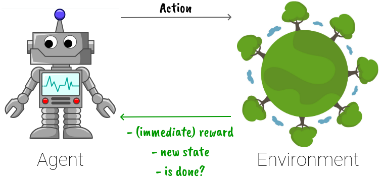
Reinforcement learning: Q Learning, Deep Q Learning introduction with Tensorflow

Reinforcement learning is different from supervised and unsupervised learning in the sense that the model (or agent) is not provided with data beforehand, however, it is allowed to interact with the environment to collect the data by itself. This learning format has some advantages as well as challenges.

Advantages:

Rather than working with a limited dataset, the agent can theoretically collect an infinite amount of data.
The agent can focus on collecting the data it feels more important.

Challenges:

It takes time to interact with the environment to get data.
Among an infinite pool of possible data, what data should the agent collect?
When the agent interacts with the environment, the data it gets is auto-correlated. If the agent is trained on this data sequentially, there would be probably some bad impacts on learning stability and convergence.

agent and environment — Agent and environment. The agent perceives the current state and takes and action. It then receives the immediate reward, the new state, and knows if the task is done.

In this blog post, we give an introduction to Q learning and its variant, deep Q learning. We also examine how they utilize the advantages and address the challenges of reinforcement learning.

Definition: On-policy and off-policy methods.

When an agent interacts with the environment, the current state, how it acts, and the result are recorded as a training data point.

On-policy methods are reinforcement learning methods that learn from the data generated by their own policy, while off-policy methods can learn from data generated from different sources. In other words, an on-policy algorithm trains itself solely on the data it gets by interacting with the environment using its policy, while an off-policy algorithm doesn’t care about if the data is generated by itself or by, say, another agent.

In simple terms, an on-policy algorithm is similar to someone who only learns from her own successes/mistakes, while an off-policy algorithm is analogous to someone who can look at others’ successes/mistakes and learn from there.

Q learning and deep Q learning are off-policy methods.

Definition: Epsilon-greedy.

Similar to humans, learning agents should also balance between exploitation and exploration. Exploitation means doing what we have known as the best given the current situation. Exploration means taking another action that is not the best to our knowledge. Exploitation’s goal is to get a good result at the moment, while exploration aims to widen our knowledge (so we may get better results for future situations). Also notice that exploitation keeps the agent active on a potential track, which addresses the question of which data should it collect (the second challenge we stated above).

Epsilon-greedy is the most simple but also very effective approach to trade-off exploitation and exploration. That is, with a chance of epsilon (0 < epsilon < 1), we explore, otherwise, we exploit.

For example, let’s say we set epsilon to be 0.2. Then, given a situation, with the probability of 20% we do a random action, while with the probability of 80% we do the best action we know so far. Note that for simplicity, in practice, exploration selects a random action from the pool of all possible actions including the action we think is the best for the current situation. Thus, the chance that action is chosen is a bit more than 80% in the above example.

Q learning

The Q learning algorithm attempts to learn a table of size (number of observations $\times$ number of actions), in which the cell (i, j) represents the quality of taking action j given the i-th situation (or state, or observation, for simplicity we use these 3 words interchangeably in this blog post).

Suppose we already have a Q-table filled with reasonable values, then given any observation, the agent knows how to react, it simply selects the action which yields the highest quality.

The question is how to learn the Q-table effectively. To do so, we rely on the Bellman equation, as below:

$Q(s, a) = r_{s, a} + \gamma \max_{a_i} Q(s', a_i)$

where:

$Q(s, a)$ is the quality of action $a$ given state $s$ , i.e. the corresponding cell in the Q-table.
$r_{s, a}$ is the immediate reward we get when doing action $a$ given state $s$ . Depending on the task to be solved and our approaches, $r_{s, a}$ can be ignored. For example, in Chess, moving a piece (action) does not necessarily incur any reward except that is the final move, so we may set $r_{s, a}$ to be 0 for some $s$ and $a$ .
$s'$ is the new state we get to after performing action $a$ in state $s$ . In Chess, $s'$ is the new board after we move our piece.
$\max_{a_i} Q(s', a_i)$ is the highest quality we can get to if we are in state $s'$ . In other words, it is the highest value in the Q-table row corresponding to the state $s'$ .
$\gamma$ is the discount factor for delayed reward. $0 \le \gamma \le 1$ . Getting the reward immediately is usually better than in the future.

The Bellman equation is thus a way to define the quality of a state-action pair given its neighbors. Notice that in the beginning, while most values in the Q-table are unknown, we know the values of some cells which correspond to the final states. In games, these final states mean the states representing the end of the game, whether we win or lose. We can mark these values as 1 if we win and -1 if we lose. Then, they act as anchor points so that we can use the Bellman equation to learn the values of its neighbors, and of its neighbors of neighbors, and so on.

In practice, for stability of training, we make use of the learning rate factor:

$Q^{\text{desired}}(s, a) = (1-\alpha) \times Q^{\text{old}}(s, a) + \alpha \times Q^{\text{target}}(s, a)$

where:

$\alpha$ is the learning rate. $0 < \alpha \le 1$ . Higher $\alpha$ means faster adaptation to new knowledge, but usually the training curve is less stable.
$Q^{\text{old}}(s, a)$ is the old value in the Q-table (“old” means before performing this update).
$Q^{\text{target}}(s, a)$ is the quality of the pair $(s, a)$ as computed using the Bellman equation at the moment. $Q^{\text{target}}(s, a) = r_{s, a} + \gamma \max_{a_i} Q(s', a_i)$ .
$Q^{\text{desired}}$ is the value we want the quality of (s, a) to be adjusted to be, given the old and target quality.

Gathering all the pieces, the learning is performed iteratively by looping the below until convergence of the Q-table:

the agent perceives the current state.
the agent selects the action using the epsilon-greedy mechanism.
the agent does the action, receives reward and new state from the environment.
the quality of the pair (state, action) is updated following the Bellman equation and learning rate.
now the current state is set to be the new state just received from the environment.

Deep Q learning

While Q learning is relatively simple and effective for small tasks, it has a vital drawback: the Q-table can be infinitely large, rendering it infeasible to compute and store. For example, Chess has approximately $10^{120}$ possible states, thus the Q-table needs about this number of rows, which is just impossible.

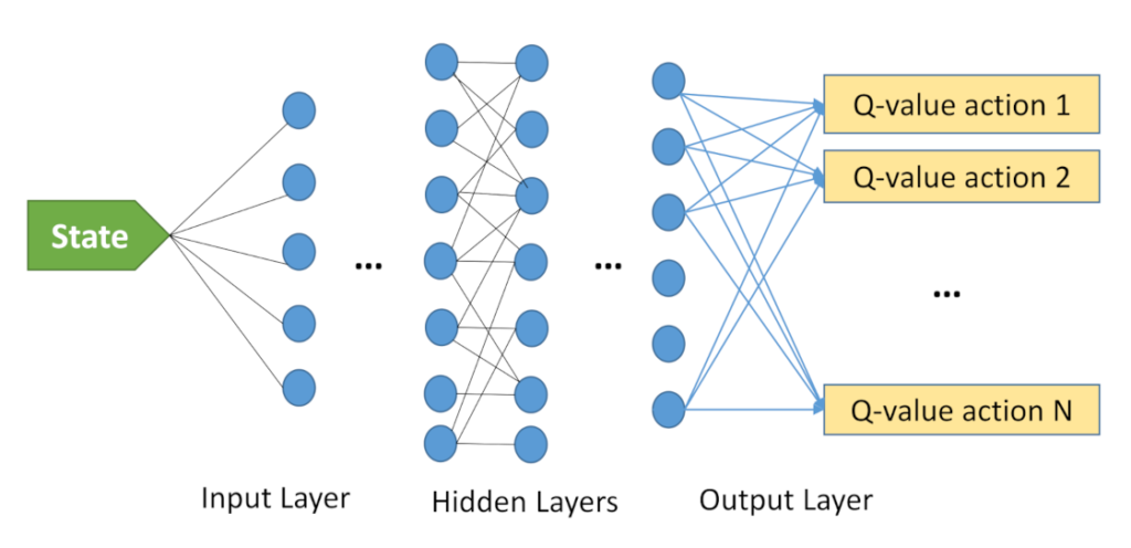
To deal with this issue, one approach is to compress the Q-table in the form of a neural network. The idea is that while there are many states, some of those states can be very similar to each other (e.g. symmetrical board in the game of Go) so compression may trade-off a bit of specificity for lots of spatial and computational gains.

The structure of the network looks like below. Input is the state, while output is the Q-values for each of the actions (given that input state).

This learning format makes deep Q learning very similar to a canonical (supervised) classification problem. It is. However, there are a few tricks that need to be introduced to make learning stable and efficient.

Definition: Experience Replay.

One of the challenges with reinforcement learning’s data generation scheme is that the data is auto-correlated, i.e. 2 data points generated at similar timestamps are highly correlated. This affects the stability of the training process, making the network hard to converge.

Experience replay means we store the generated data in a pool, and for each time we want to train the network, we sample a random minibatch from this pool. This handles the auto-correlation problem because the data to be fed to the network is not correlated anymore.

Moreover, to keep the pool competent, i.e. the data in the pool is relevant for training the current network, we discard too-old data points when new data points arrive. In practice, it is sufficient to structure the pool as a deque with a fixed maximum length. Thus, when new data is pushed, the oldest data is automatically popped to ensure the deque size does not exceed the predefined length.

Definition: deep Q learning loss function.

While experience replay bridges the gap between reinforcement learning and supervised classification, the loss function drives them apart. If you have some experience with neural network classification, you know the cross-entropy loss function penalizes all the outputs returned by the network. That is, all values coming out from the output layers are compared to some ground truths to calculate the loss. This is a bit different with a deep Q network, in which only one value in the output, the one corresponding to the intended action, is taken into account for computing the loss.

Let us take an example.

Suppose that in our task, a state is represented by a list of 4 numbers, and there are in total 3 possible actions (denote the actions as 0, 1, and 2). Assume the discount factor $\gamma = 0.8$ and the learning rate $\alpha = 1$ . An experience is a tuple consisting of a state, an action, the immediate reward for taking this action is this state, the new state incurred by taking this action in this state, and a boolean value specifying if the new state signifies the end of the task.

Say we have an experience with state [0.1, 2, -3, 2.5], action 2, reward 5, and new state [-2.2, 4, 2, 1.1]. Now, by feeding forward the state [0.1, 2, -3, 2.5] to the network, we receive the output [-2, 1.6, 0.2]. By feeding forward the new state [-2.2, 4, 2, 1.1] to the network, we receive [2.3, 1.5, 0.8].

The current quality of taking action 2 in the state is $Q(s, a) = 0.2$ , as seen from the output above. The target quality of taking the same action 2 in the state is, as computed by the Bellman equation, $Q^{\text{target}} = 5 + 0.8 \times 2.3 = 6.84$ . Since $\alpha = 1$ , we have $Q^{\text{desired}} = 6.84$ .

The loss is then computed by comparing 0.2 and 6.84. For example, if we further assume the loss function is Mean squared error, then $loss = (6.84 - 0.2)^2 = 44.0896$ . Notice how the loss only depends on 0.2 while the network outputs [-2, 1.6, 0.2] for the state. This is in contrast with traditional classification problems, in which all output values are needed for the loss.

Definition: the target (or frozen) model.

This is how we defined the Bellman equation in the above sections:

$Q(s, a) = r_{s, a} + \gamma \max_{a_i} Q(s', a_i)$

There is a problem: when we update the network using this equation, not only the predicted output but also the target change (because both are computed from this network). This makes the learning process more like a never-ending chase, the predicted output cannot catch the target because the target is also moving. Thus, it is hard to converge.

In practice, researchers realize that it is more beneficial if we don’t update the network (for computing the target) that frequently. They suggest copying the main network to a target network (i.e. we have 2 networks) and only update this target network after a number of training steps rather than after every training step. This target network is also sometimes called the frozen network.

As we adapt this suggestion, the Bellman equation is rewritten as:

$Q(s, a) = r_{s, a} + \gamma \max_{a_i} Q^{\text{frozen}}(s', a_i)$

where the only difference is that $Q^{\text{frozen}}(s', a_i)$ replaced $Q(s', a_i)$ . This means this quality is computed by the frozen network, not the main network.

A deep Q model with this frozen network integrated is sometimes called a fixed deep Q network.

Definition: double deep Q network.

Let us copy the above Bellman equation for the fixed deep Q network here:

$Q(s, a) = r_{s, a} + \gamma \max_{a_i} Q^{\text{frozen}}(s', a_i)$

For double deep Q network, it is changed to:

$Q(s, a) = r_{s, a} + \gamma Q^{\text{frozen}}(s', \arg \max_{a_i} Q(s', a_i))$

So the only difference is we don’t fully rely on the frozen network to compute the target Q-value. Instead, we use the main network to find the best action given the new state $s'$ and then compute the frozen Q-value of the pair ( $s'$ , that best action). This is to handle the problem called Maximization Bias, i.e. the Bellman equation always selects the action whose Q-value is the highest, but this “high value” may just be due to chance. Take the figure below as an example.

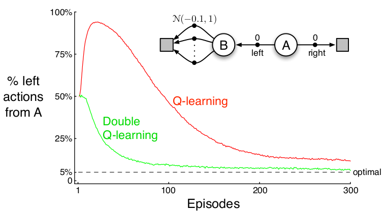
Maximization bias - RLBook chap 6.7 — Maximization Bias problem. The figure is taken from the RL book by Sutton and Barto.

Let’s look at the decision process at the top right first. In this setting, the agent starts from A and has 2 possible actions: going left or right. If it goes right, it gets a reward of 0 and immediately reaches a terminal state. If it goes left to B, it also gets a reward of 0, but from B it can only go left using one of several actions, the rewards resulting from these actions are normally distributed with mean -0.1 and variance 1. Thus, in fact, from A, to go right is the better option. However, the agent may mistakenly want to go left because N(-0.1, 1) may give some positive values, and suddenly from A going left to B and then from B select the best action will result in a positive reward overall.

Now, look at the plot. This plots how Q learning and double Q learning favor the left action after being trained for some number of episodes, with the current epsilon = 0.1. With this epsilon, an ideal agent would select the left action with the probability of 5%. The double Q learning model does well on approaching this ideal number, but the original Q learning model cannot.

We get a better outcome from the double Q learning model since the learning weights do not only depend on the (monopoly) frozen network, which in that case can manipulate the whole process.

Note that there are different implementations of the double deep Q network. Here, we introduce the version that is very similar to the fixed deep Q network. Another version of the double deep Q network uses 2 neural networks interchangeably, i.e. no separation between the main and the target networks. Although not described here, the code for this implementation can be found in the repository at the end of this blog post.

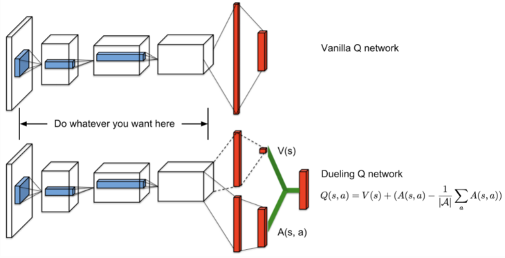
Definition: dueling deep Q network.

The dueling deep Q network decomposes the Q-value Q(s, a) into V(s) and A(s, a).

$Q(s, a) = V(s) + A(s, a)$

where:

$V(s)$ is the value of state $s$ . $V(s)$ represents how prestigious the state $s$ is regardless to any action. In other words, we can say $V(s)$ is the average Q-value of state $s$ with any action. $V(s) = \frac{1}{N} \sum_{i=0}^{N-1} Q(s, a_i)$ , where $N$ is the number of actions.
$A(s, a)$ is the advantage of taking action $a$ given state $s$ compared to the average. Following this formulation, we have $\sum_{i=0}^{N-1} A(s, a_i) = 0$ .

The separation of V and A is a good idea as V can be computed with efficient use of data. For example, say we have 1000 data points for 10 observations and 4 actions, then the average sample per (s, a) pair is $\frac{1000}{10*4} = 25$ . So for each Q(s, a) and A(s, a), we have on average 25 data points. However, as V only depends on the state but not the action, each V(s) has $\frac{1000}{10} = 100$ data points to compute from, which makes the estimation of V more accurate. And since V is more accurate, $Q = V + A$ would also be more accurate.

As an implementation detail, to make sure $\sum_{i=0}^{N-1} A(s, a_i) = 0$ , we replace the original formula $Q(s, a) = V(s) + A(s, a)$ with $Q(s, a) = V(s) + (A(s, a) - \frac{1}{N} \sum_{i=0}^{N-1} A(s, a_i))$ .

screenshot from 2021 09 08 10 30 29 — Comparison of vanilla Q network with dueling Q network. The figure is taken from Wang et al.

If you have read up until this point, I guess you probably have in mind some ideas of how to train a deep Q network. Apart from the adjustments we elaborated on above, the remaining process is basically the same for any classical classification network.

Code: A working example for deep q learning can be found in my git repository. The notebook implements and trains a simple deep Q network for the CartPole game from OpenAI with the help of TensorFlow.

screenshot from 2021 09 06 22 28 57 — The CartPole game.

References:

An introduction to Q-Learning: Reinforcement Learning, floydhub
Deep Q-Learning Tutorial: minDQN, medium
How exactly to compute Deep Q-Learning Loss Function?, StackExchange
Experience Replay, PapersWithCode
What is “experience replay” and what are its benefits?, StackExchange
Deep Q-Learning, Part2: Double Deep Q Network, (Double DQN), medium
Q-targets, Double DQN and Dueling DQN, theaisummer
Improvements in Deep Q Learning: Dueling Double DQN, Prioritized Experience Replay, and fixed…, freecodecamp

Tung M Phung's Blog

Reinforcement learning: Q Learning, Deep Q Learning introduction with Tensorflow

Q learning

Deep Q learning

Leave a ReplyCancel reply