The Transformer neural network architecture

The Transformer network has made a revolutionary breakthrough in Natural Language Processing. Since its debut in 2017, the sequence-processing research community has been gradually abandoning the canonical Recurrent neural network structure in favor of the Transformer’s encoder-decoder and attention mechanisms. In this blog post, we will walk through its components to understand how it works and what made it a great success.

Overall structure

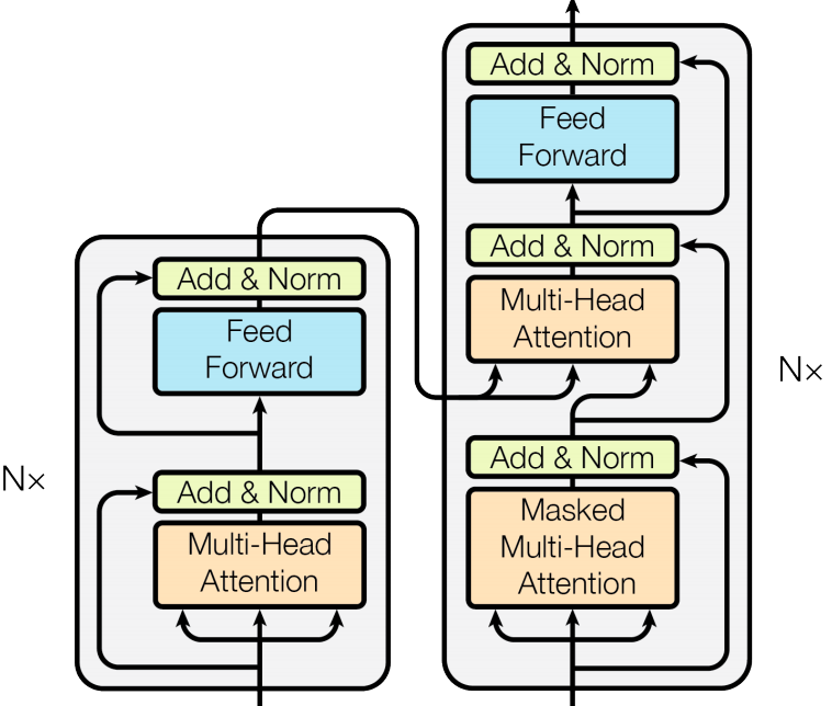
The original paper [1] provides a condensed view of how the Transformer looks like (Figure 1).

This flow-graph does a great job to showcase a summary of the pieces that constitute the Transformer, those are:

Sequence Embedding and Positional Encoding

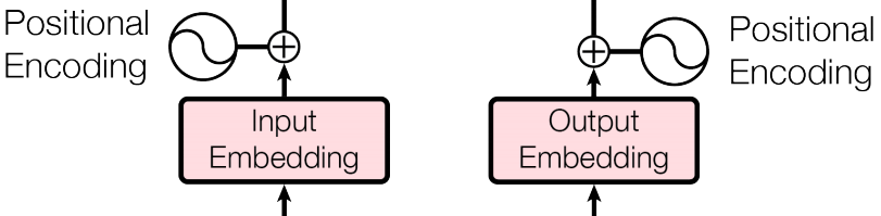
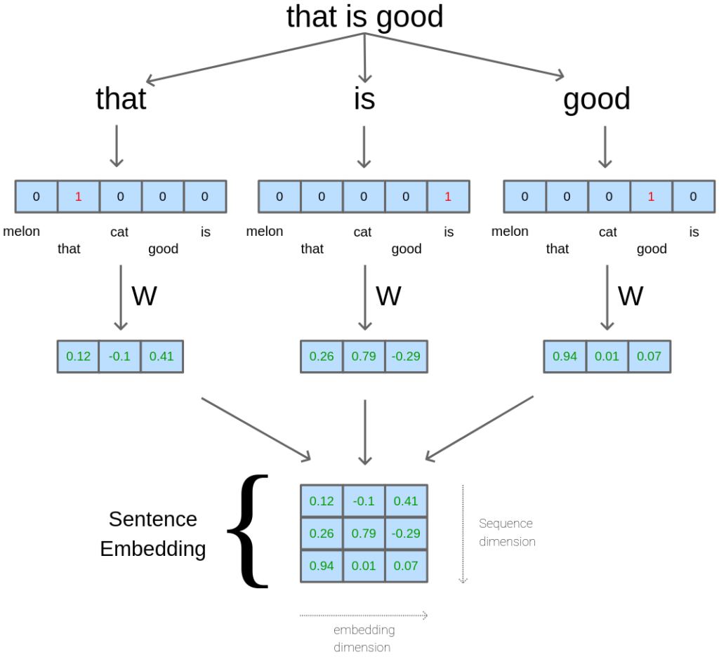
Sequence Embedding

The Transformer was originally proposed to work with Natural Language Processing (NLP) tasks, which often takes as input a sequence of words (or say a sentence, which contains an arbitrary number of words). Normally, each word in the sentence is transformed into a vector of numbers representing that word in the semantic space. Words with similar meaning are expected to stay closer to each other in that space (while closeness is often measured by the dot-product of 2 vectors). A sentence (or a sequence of words) is then denoted by the concatenation of its words’ vectors. For example, for a sentence of 12 words, each word is mapped to a vector space of dimension 512, then the sentence corresponds to a vector of 12×512 = 6144 numbers, or equivalently a matrix with size [12, 512]. We say that a big vector (or matrix) is the embedding of the given sentence (or sequence) – Figure 3.

In particular, given a sentence, each word is converted to an index number in the vocabulary (of size 10000), this number is one-hot encoded, then, the encoding is transformed into an embedding vector (of size 512) by a dense linear mapping (i.e. the embedding weight-matrix). In the Transformer, the same weight-matrix is shared between the two embedding layers and the pre-Softmax transformation (transposed). This trick was proposed in [10].

Positional Encoding

Before the bond of Transformer, almost all modern NLP problems are attempted by some types of Recurrent neural network models (LSTM or GRU, for example). With these networks, for each input sequence, the words are fed one-by-one. That is, for example, for an input sentence “That dish was good but a bit too salty” that has 9 words, each of these words, from “that” to “salty” is given to the RNN in that order. In that way, the RNN has a clear understanding of the order of words, which plays a very important role in the meaning of the sentence.

However, the Transformer doesn’t consume the words sequentially but rather takes the whole sequence at once. This makes a significant effect on training time since it allows parallel processing, which results in a substantial boost in speed, yet, the problem is that the order of words is not well perceived by (the attention layer of) the model. (As we will see in the later sections, the output of the attention layer is basically a weighted sum, and it is trivial that the result of a summation has no dependency on the order of the operands.) To address this problem, the authors’ solution is to push the information about the order of words into the input to be given to the Transformer.

Naturally, one would do that by simply appending the absolution position index to the input embedding. For example, in the embedding of the sentence above, instead of the embedding matrix of size [12, 512], we attach to each word one more value that represents its position (from 1, 2, 3, … to 12), making the matrix size [12, 513]. In general, this means we attach an increasing and equal-distance value to consecutive words. However, this approach has a problem with extrapolation. In cases when a test input sequence is longer than all training sequences, the model might struggle with position values that it has never seen before.

Another tactic would be to make the position values relative. Put it differently, we make the distance between consecutive words equal but relative to the length of the sentence. For example, with a sentence of 12 words, the positions would be . This solves the above problem with absolute distance, however, it also has a drawback that sentences with different lengths will have different position values, which results in undesired inconsistency in positional encoding.

The authors propose a method that attempts to solve both of these issues, i.e. the sin-cos encoding. The positional encoding has the same size as the embedding (512 dimensions) and is computed using the following formula:

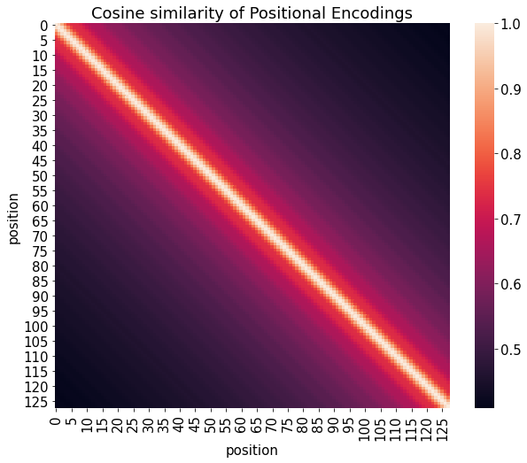
where is the position of the word in that sentence, is the dimension (i.e. runs from 0 to 511), and is the dimension size ( = 512). This positional encoding is then added directly to the embedding values (they have the same dimensions), rather than being concatenated. Figure 4 shows how the positional encoding looks like for 128 positions and 512 dimensions.

Here are the advantages of this method:

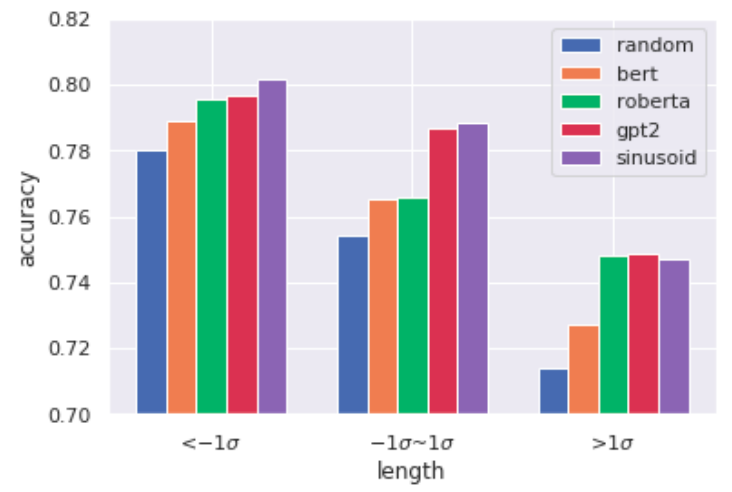
In practice, the performance of this sinusoidal PE is very competitive. As shown in [15], it has even stronger positional effects than other newer alternatives proposed with the state-of-the-art BERT, RoBERTa, and GPT-2. The small figure below is taken from that paper. It implies that sinusoidal PE achieves good accuracy regardless of input text lengths.

There is another reasoning for adding the positional encoding to the text embedding (rather than concatenating), which will be discussed later when the attention mechanisms have been explained (here).

The Encoder-Decoder scheme

Using the Encoder-Decoder structure has been a standard for seq2seq tasks (i.e. input a sequence and output another sequence with possibly different length) long before the time of Transformers. In this formulation, the input for the encoder is the original input, while to be fed into the decoder is the output of previous phases. For example, in Machine Translation, suppose we want to train a network to translate from English to German. It will work as follow:

• First, the full English sentence is fed into the encoder while a null string is taken in by the decoder. The encoder processes the sentence, extracts its meaning to a vector, and passes that vector to the decoder, who takes it together with a null string to output the first German word.
• Second, the encoder stays still, it doesn’t have to do anything more but just keep passing the vector it had from the first step to the decoder, the decoder takes that vector and the sequence of words it has outputted before to process and output the second word.
• And so on, the decoder gets the semantics of the English sentence from the encoder, it also considers its outputted words from previous steps to guess the next word, until it feels the translation is completed.

In Transformer, both the encoder and the decoder are composed of 6 chunks of layers. Figure 6 shows only one chunk of encoder and decoder, the whole network structure is demonstrated in Figure 7.

Attention

Attention stands as the heart of the Transformer. If you have no idea about what Attention in neural networks is, we have a full article dedicated to your information here. In short, given a context, the Attention mechanisms help the network locate which parts of the input that it should focus on (i.e. put more weights on) to generate the right output.

Scaled Dot-Product Attention

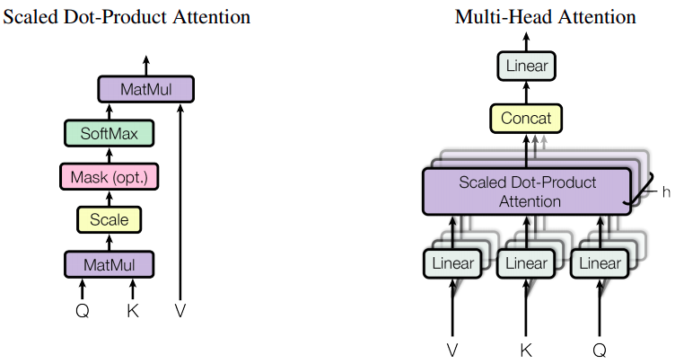
In the Transformer, there are 3 slightly different types of Attention (Figure 8). The grey-bounded is the Encoder attention, the purple-bounded is the decoder attention, and lastly, the green-bounded is the encoder-decoder attention (since it takes input from both the encoder and from the lower layer of the decoder).

We can see that there are 3 arrows pointed to each Attention layer, which means they take in 3 inputs, namely the Query (Q), the Key (K), and the Value (V). This concept is borrowed from the field of Information retrieval, that is, say, given a set of many key-value tuples, find the value(s) corresponding to the key(s) that match a query the most. For example, suppose you have a keyword (query) “Transformer network” and you want to search on Google for the texts or papers (values) whose headers or titles (keys) best match your query.

In the Transformer, a specific type of Attention is used, the Scaled Dot-Product Attention:

Attention(Q, K, V) = softmax()V (1) (*caveat)

where Q, K, V are as we have stated, and is the number of dimensions for the key K. Specifically, gives the similarities between Q and each key (vector) from matrix K (K is a matrix where each row represents a key). The softmax function is applied to normalize all the similarities (i.e. the attentions) so that they sum to 1. The result is then multiplied by the matrix V which containing the corresponding values, so the more similar Q to a key, the more similar the returned Attention to the corresponding value of that key. The division by is what makes this a Scaled Dot-Product rather than the canonical Dot-Product. This is an adjustment made by the authors of the Transformer to neutralize of bad effect of long sentences:

We suspect that for large values of , the dot products grow large in magnitude, pushing the softmax function into regions where it has extremely small gradients. To counteract this effect, we scale the dot products by .

From [1].

In case of the encoder attention(, remember that its input is the actual input sequence), the problem is translated to: given a sequence of words, for each word in that sequence (query), find the words in the same sequence (values) that themselves (keys) match the word (query) the most. This may look confusing, however, the idea is as simple as we let all query, key, value be the input sequence. This is also called Self-Attention. Look at Figure 9 for an illustration.

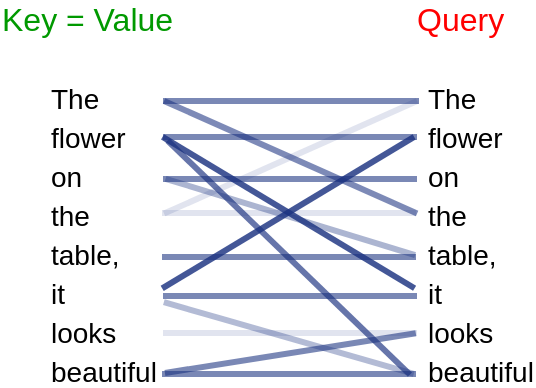
The objective of this encoder attention layer is to find, for each word, which other words in the same sentence are most related to it. For instance, in Figure 9, the word “it” is related to itself and even more related to “flower”, so when there is a need to predict something about “it”, the model knows it should get information from “flower”. Say, for some reason, the model needs to know where “it” is, since it already knew the “flower” is on the table and “it” refers to “flower”, the model can answer that “it” is on the table.

The decoder attention layer works almost exactly the same, with the exception that future words are masked. That means, say, when the model learns to predict the i-th words in the output, it is limited to know only the first (i-1) words of the output, but not the i-th word and further. We only need this mask on the first decoder chunk.

The encoder-decoder attention layer (the green-bounded box in Figure 8), on the other hand, takes K and V from the encoder (K = V) and Q as the output of the last layer in the decoder. The goal of this layer is: for the sequence of words the model has outputted (Q), find the best attention distribution that it should use to predict the next word (i.e. find how it should attend to the input’s semantic vector to best predict the next word).

Note that for practical purposes, you should keep in mind how we actually call formula (1). We don’t call Attention, but Attention, where , , and are 3 learned matrices of the attention layer.

Another important point is that the output of an attention layer is actually not the attention itself, but rather the attention glimpse (i.e. the view the model look with attention taken into account). The actual attention distribution in (1) is softmax() without multiplying to V.

About the actual matrix size:

• 
• 
• 
• Attention

where is the number of tokens in the query, is latent dimensions ( = 512), is the number of tokens in the input, and is the latent dimension of attention.

Multi-Head

The prefix “Multi-Head” sounds fearsome, but it just means a bag of Attention layers (instead of just one) are working simultaneously and independently. The results of these Attention layers are then concatenated and pushed forward to a dense Linear layer, whose role is to aggregate all attention glimpses into one. (Figure 10, right).

It is also helpful to mention that the number of learnable parameters in a Multi-Head Attention layer may or may not increase with the number of heads, depending on the implementation. In PyTorch, adjusting heads does not affect the number of parameters since the size of matrices , , and ( is an iterator over all heads) are adapted to (divided by) the number of heads [12].

The reasoning behind Positional Encoding and Attention

Normally, one would expect to see the Positional Encoding being appended to the semantic vector of the input rather than directly added to it. We have given one reason why adding should work above. In addition, Pappypapaya also has an interesting view supporting this operation [6]. We will try to re-interpret his idea here:

Basically, in Dot-Product Attention, we want the attention distribution which is determined by

.

So, equivalently, we just want the model to learn a matrix , which will answer the question: how should the attention be distributed to K given Q?

Now, when we add the positional encoding E of Q and F of K to the formula, that would be:

Thus, besides asking how should the attention be distributed to K given Q?, now we also ask: how should the attention be distributed to K given position E of Q? how should the attention be distributed to position F of K given Q? how should the attention be distributed to position F of K given position E of Q?

The first additional question, how should the attention be distributed to K given position E of Q?, is very intuitive and supports the rationale behind adding PE to embedding very well. However, the other two seems not so persuasive, maybe this could serve as the start of a research question.

Residual learning and Shortcut connection

Residual networks and Shortcut connections are ubiquitous in all types of deep learning models, thanks to Kaiming He et al. with [11]. The concept is very simple but surprisingly effective: by applying element-wise additions from outputs of lower layers to some-level-higher layers, it becomes feasible to train much deeper networks, making the performance vastly increased. Figure 11 briefly illustrates how it works.

Layer Normalization

Layer Normalization was not something people talked about before the appearance of the Transformer. However, from that time up, LayerNorm has become the most frequently used normalization method in NLP. The formulation of LayerNorm is rather simple (it inherits mostly from the predecessor BatchNorm), for each input sequence:

• Step 1: every value is standardized (i.e. demeaned and divided by standard deviation).
• Step 2: the values are then affine-transformed by 2 learned scalars and :

where is the final normalized value and is the standardized value obtained from step 1.

The most important effects LayerNorm brings in this case are probably making the optimization function smoother and mitigating the gradient vanishing/exploding problems.

LayerNorm along with BatchNorm and other normalization methods are discussed in detail in another article, Deep Learning normalization methods.

Code

Major deep learning frameworks like PyTorch and TensorFlow all actively support with implementations of the Transformer. A short, worked example on how to use the Transformer for Neural Machine Translation (NMT) can be found in this repo.

Final words

The Transformer made a revolution, neither because it performs better than other architectures at its birth time, nor its debut the amazing Attention mechanisms. In fact, the Attention was proposed many years ago, the Encoder-Decoder stack was also used widely long before. What makes the Transformer special is that it eliminates the use of Recurrent layers and uses only Attention to compensate for that loss. From this breakthrough, almost all new-born state-of-the-art language processing models (e.g. BERT) are based on the structure of the Transformer. While many people say that RNNs are effectively dead, some even say that Convolutional neural networks (CNNs) are also on the edge [13] [14]. Let’s see what’s going on next.

References:

[1] Attention is all you need, Vaswani et al., paper
[2] Transformer: A Novel Neural Network Architecture for Language Understanding, Jakob Uszkoreit, blog
[3] Attention? Attention!, Lig’Log, blog
[4] Transformer neural network, Thomas Wood, blog
[5] Deep learning, the Transformer, blog
[6] Why positional embedding works and why adding instead of concatenating, pappypapaya, answer
[7] Linear Relationships in the Transformer’s Positional Encoding, Timo Denk, blog
[8] What do Position Embeddings learn? Yu-An Wang and Yun-Nung Chen, paper
[9] Rethinking Positional Encoding in language pre-training, Guolin Ke et al., paper
[10] Using the Output Embedding to Improve Language Models, Press & Wolf, paper
[11] Deep Residual Learning for Image Recognition, Kaiming He et al. paper
[12] Count the number of parameters in Multi-Head Attention, StackOverflow and PyTorch
[13] Stand-Alone Self-Attention in Vision Models, Ramachandran et. al.: paper
[14] On the relationship between self-attention and convolutional layers, Cordonier, paper
[15] What Do Position Embeddings Learn?, paper