Deep Learning normalization methods

It has been shown from 1998 [1] that normalization helps with optimizations, making the neural networks converge faster. However, not until 2015, when Batch Normalization [2] is published that this research direction is extensively explored by the community. Since then, many other normalization schemes have been proposed, with Weight Norm [3], Layer Norm [4], Instance Norm [5], and Group Norm [6] being the ones that get the most attention from the public. In this article, we will introduce these techniques and compare their advantages and disadvantages over each other.

Definitions

Batch Normalization

With Batch Norm, all data points of the same input mini-batch are normalized together per input dimension. In other words, for each dimension of the input, all data points in the batch are gathered and normalized with the same mean and standard deviation. Below is the transformation of BatchNorm for each separate dimension of the input x.

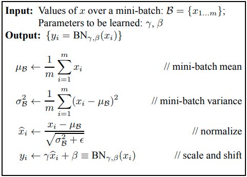
Batch Norm transformation — *The transformation of BatchNorm, taken from its original paper.*

Note that in the case of convolutional layers, the “dimension” is perceived as the channel dimension, while in feed-forward layers, it is the feature dimension. With that to say, for example, the input data is normalized separately for each channel in a convolutional layer.

In the above algorithm, $\mu_B$ is the sample mean of the m data points in the minibatch, $\sigma_B^2$ is the corresponding sample variance. $\gamma$ and $\beta$ are 2 parameters that are learned during Back-propagation.

A throughout discussion about BatchNorm and why it works is given in our another blog post.

Weight Normalization

Unlike BatchNorm which normalizes the neuron’s value before or after activation, WeightNorm tends to normalize the weight vectors. Even more interestingly, WeightNorm decouples the norm and value of the weight vectors. Thus, instead of learning a weight vector $w$ , we instead learn a scalar $g$ – the norm (or informally the strength, the magnitude of the weight vector) and a vector $v$ – the direction of the weight vector.

$\begin{aligned} w = \frac{g}{||v||} v \end{aligned}$

While the weight vectors $w$ are used in the forward phase as usual, the backward optimization optimizes the values of $g$ and $v$ . Intuitively, this decoupling makes the norm of the parameters (i.e. the weights) more explicit,

Layer Normalization

LayerNorm uses a similar scheme to BatchNorm, however, the normalization is not applied per dimension but per data point. Put it differently, with LayerNorm, we normalize each data point separately. Moreover, each data point’s mean and variance are shared over all hidden units (i.e. neurons) of the layer. For instance, in Image processing, we normalize each image independently of any other images, the mean and variance for each image is computed over all of its pixels and channels and neurons of the layer.

Below is the formula to compute the mean and standard deviation of one data point. $l$ indicates the current layer, H is the number of neurons in layer $l$ , and $a^l_i$ is the summed input from the layer $l-1$ to neuron $i$ of layer $l$ .

Using this mean and standard deviation, the subsequent steps are the same as with BatchNorm: the input value is demeaned, then divided by standard deviation, and then affine transformed with learned $\gamma$ and $\beta$ .

Instance Normalization

InstanceNorm is also a modification of BatchNorm with the only difference is that the mean and variance are not computed over the batch dimension. In other words, only the pixels in the same image and the same channel share the mean and variance of normalization. With such a restricted normalization range, the use of InstanceNorm seems to be limited in computer vision when the input is image data.

The formula is:

$\begin{aligned}& \mu_{ti} = \frac{1}{HW} \sum_{l=1}^W \sum_{m=1}^H x_{tilm}, \\& \sigma_{ti}^2 = \frac{1}{HW} \sum_{l=1}^W \sum_{m=1}^H (x_{tilm} - \mu_{ti})^2, \\& y_{ijk} = \frac{x_{tijk} - \mu_{ti}}{\sqrt{\sigma_{ti}^2 + \epsilon}}\end{aligned}$

with H, W being the height and width of the input image. t, i, l, m are the iterators over images in the minibatch, channels, width, and height of the images, respectively. j and k also iterate over the width and height.

Group Normalization

GroupNorm is a trade-off between LayerNorm and InstanceNorm. Note that the major difference between LayerNorm and InstanceNorm is that LayerNorm does take the channel dimension into computation while InstanceNorm does not. GroupNorm, on the other hand, groups channels into groups and normalize inside each group. The batch dimension is still not used (only BatchNorm normalizes over the batch dimension).

Normalization methods comparison

In [6], the authors give a simple visualization showing the major differences among the 4 normalization methods (except WeightNorm):

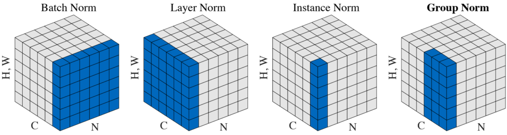
The major differences among 4 normalization methods. The blue pixels are normalized by the same mean and variance, computed on the values of these pixels.

As a reminder, we recall that these 4 methods share the same structure: each value is standardized (i.e. demean and divide by standard deviation) and then reconstructed with an affine function on 2 learned scalars $\gamma$ and $\beta$ .

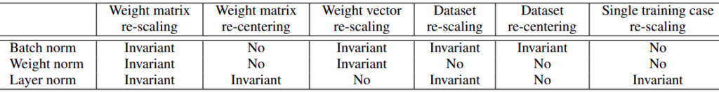
In [4], there is a comparison of invariance properties under BatchNorm, WeightNorm and LayerNorm:

Invariance of normalization methods. — Invariance properties of normalization methods.

Advantages and Disadvantages

Normalization methods, in general, help with speeding-up optimization to have the network converge faster. Furthermore, they have a substantial effect on controlling gradient vanishing and exploding. Below, we examine other properties that make each of the scheme unique.

Batch Normalization

BatchNorm reduces the bad effects of an inappropriate learning rate. Thus, it is possible to apply a higher learning rate to make the network train faster.
The regularization BatchNorm produces is distinctive and is not compensable by other standard regularization techniques such as dropout and weight decay [7]. This effect is highly appreciated, especially in the field of computer vision.
Since the normalization of a data point is dependent on other data points in the same minibatch, the transformation is not stable and deterministic. This is both good (it engages noise for regularization) and bad (prone to error, affected by outliers, etc.)
For cases when the batch size is small (e.g. online learning, large distributed models, high-resolution input), the noise is dominant and greatly affects model performance.
How to use BatchNorm in Recurrent neural networks is not straightforward with regards to variable-sized input (i.e. different data points in one minibatch may have different sequence lengths).

Up to the moment (early 2021), BatchNorm is usually used in state-of-the-art deep vision networks (e.g. EfficientNet).

Weight Normalization

The skeleton of WeightNorm is different from the other methods, this alone is enough to make it unique. Since WeightNorm normalizes the weights, not the values at the neurons, it is computationally cheaper when being applied on convolutional layers, where there are much fewer weights than neurons.
It has a similar characteristic as BatchNorm, which is the ability to handle large learning rate effectively.
Parameters need to be initialized more carefully. With BatchNorm, parameter initialization is more care-free.
WeightNorm alone performs worse than BatchNorm (shown in the original paper [3]). However, also in [3], the combination of WeightNorm and mean-only BatchNorm outperforms BatchNorm.
The experiments in [7] indicate that although WeightNorm gives smaller training error, its testing error is much higher than with BatchNorm.

Layer Normalization

LayerNorm is deterministic in the sense that its normalization on a data point does not depend on other data points (compared to BatchNorm, which is not).
LayerNorm can be applied to Recurrent layers without any modifications. Since it normalizes over all dimensions except the batch dimension, LayerNorm is the method with the most number of points that share the same $\mu$ and $\sigma$ that can be simply applied to recurrent layers.
LayerNorm doesn’t have the special regularization effects that BatchNorm has from normalizing across data points.

Currently, many of the state-of-the-art NLP networks are using LayerNorm (e.g. BERT and its variants, Megatron-LM).

Instance Normalization

InstanceNorm removes the effect of contrast in images (thus the authors also call this Contrast Normalization [5]). This is beneficial in some specific applications, such as image stylization [5] and image dehazing [9].
Most of the regularization effects are also removed by InstanceNorm, making it less effective in general.

Group Normalization

GroupNorm achieves similar performance to BatchNorm when the batch size is medium or high, and gets much better results compared to BatchNorm when there are fewer instances in each batch [6]. This makes GroupNorm a potential replacement for BatchNorm in simple usage.

Final words

We have discussed the 5 most famous normalization methods in deep learning, including Batch, Weight, Layer, Instance, and Group Normalization. Each of these has its unique strength and advantages. While LayerNorm targets the field of NLP, the other four mostly focus on images and vision applications. There are, however, other similar techniques that have been proposed and are gaining attention from the public, for instance, Weight Standardization, Batch Renormalization, and SPADE, which we hope to cover in the next articles.

References:

[1] Efficient BackProp: paper
[2] Batch normalization: paper
[3] Weight Normalization: paper
[4] Layer Normalization: paper
[5] Instance Normalization: paper
[6] Group Normalization: paper
[7] Compare BatchNorm and WeightNorm: paper
[8] The number of parameters in a convolutional layer: answer
[9] Instance Normalization in Image Dehazing: paper
[10] Why BatchNorm per channel in CNN: answer

Tung M Phung's Blog

Deep Learning normalization methods

Definitions

Batch Normalization

Weight Normalization

Layer Normalization

Instance Normalization

Group Normalization

Normalization methods comparison

Advantages and Disadvantages

Batch Normalization

Weight Normalization

Layer Normalization

Instance Normalization

Group Normalization

Final words

Leave a ReplyCancel reply