
Networks with Attention mechanisms are currently the state-of-the-art in Natural language processing (and maybe as well in Computer vision in the near future, Ramachandran et. al.). In this article, we attempt to present a first intuition on how Attention works and provide a minimal code-example that builds, trains, and evaluates a prototype Attention on a toy problem.
Attention
Similar to in real-life, the Attention in neural networks also refers to the most important details one should focus on (or attend to) in order to solve a given task. For example, suppose our model needs to predict the next word in the following paragraph:
The cat sitting on the table is so cute. This one here is also …
What word should be filled in the blank? Some candidates should be adorable/cute/sweet. Alternatively stated, the word to be chosen should be an adjective and have a similar meaning to cute. We know that by analyzing the given two sentences, but not every word in the two sentences has the same importance. That is, the most crucial words that affect how our (and our model’s) prediction are marked bold below:
The cat sitting on the table is so cute. This one here is also …
The is makes us think that the answer must be an adjective, the also implies that the answer should be similar in meaning to a previous adjective, and that adjective turns out to be cute. The other words do give us some context and help us understand the whole situation, however, it is clear that we depend mostly on these 3 keywords to determine our answer. Literally, for this predictive problem, we pay more Attention to cute, is, and also. The goal of introducing Attention in Deep learning is to teach the machine where to pay attention to, given its purpose and context.
Another example can be given in the problem of caption generation for images. In the influential paper Show, Attend and Tell, Kelvin Xu et. al. introduce Attention to a Recurrent neural network to generate captions for images. The words of the caption are generated one-by-one, for each word, the model pays attention to a different part of the image.
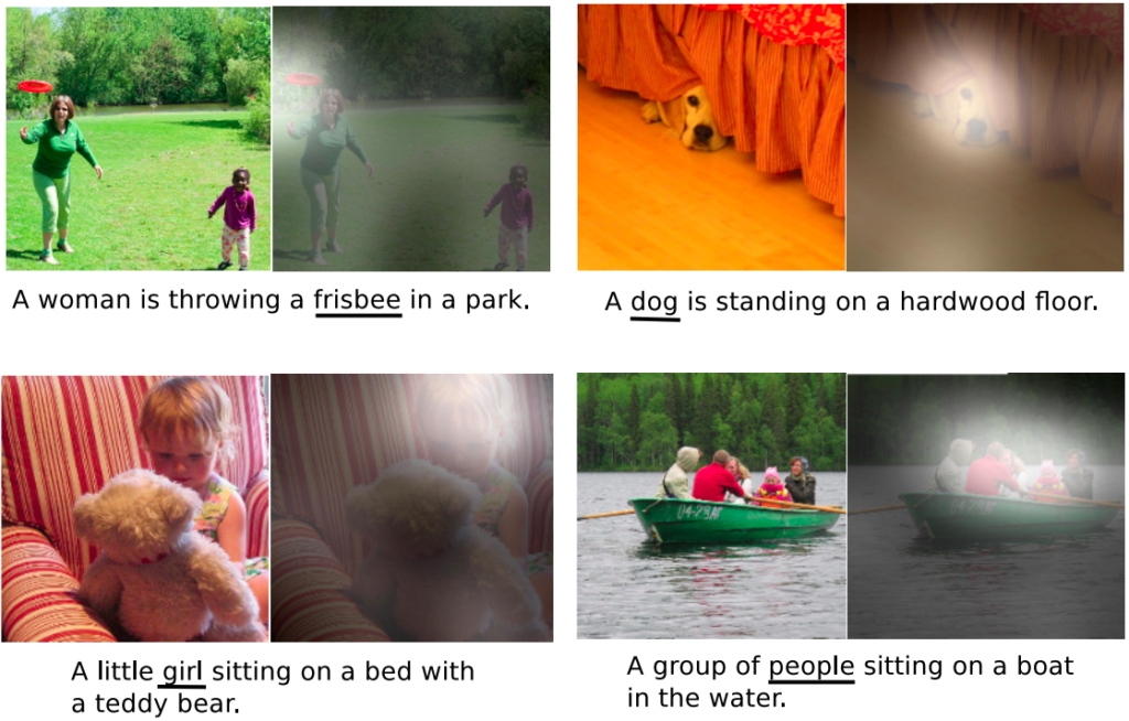
The figure above illustrates their result. The underlined words are the words that the model generates at that step, the brighter regions show where the model attends to generate those words.
The Attention function
The research community has discovered a dozen of different Attention functions. Within this post, we examine a simple formula, as described next. Intuitively, given a context c, the Attention a to the input x has the form:

where f is an Attention function that, given a context, it returns how the Attention should be distributed to the values of the input. In the above language example, the context is the inputs itself, that is, given the sequence of words The cat sitting on the table is so cute. This one here is also (context),  should produce the Attention that the model should give to that same sentence (input) to guess the next word. In the image examples, the context is the combination of the input image and the text that has been generated so far. The resulting Attention a has the same size as the input x, and each value in a is in the range from 0 to 1, with 0 indicating no attention should be given to that position, while 1 implies giving attention to it as much as you can. We also call a the Attention distribution. This Attention distribution is then used to filter the input:
g = x  a
a
means the element-wise multiplication. g is the attention glimpse (this notation is given by Kosiorek in his post), which represents how the model sees the input x with attention a. After this transformation from x to g, some values in x may be transferred to g nearly unchanged, given the values of a in these positions are near 1 (meaning fully attention), some other values may be forced to zeros if the values of a in those positions are approximately 0 (meaning no attention). From this point on, the model should only process on g but not on x anymore.
The only remaining problem is how to define the attention function  and how to train f’s parameters so that it will give the most meaningful Attention distribution for all given contexts. Since we don’t know how the ideal Attention function looks like, a solution is to approximate it using a neural network. Remember that the original purpose of neural networks is to approximate hidden functions, normally we use them to approximate the function of responses given features, now we create a network to approximate attention given contexts.
For the sake of understanding Attention, we will generate a synthesis dataset and train a network to estimate its Attention function.
A simple code example
In this example, we will build an Attention neural network using PyTorch.
import torch
import torch.nn as nn
import torch.nn.functional as F
import torch.optim as optim

import numpy as np

import matplotlib.pyplot as plt
from tqdm import tqdm
First, let’s generate a synthesis dataset, whose input data is of sequential type. There will be 10.000 data points, each is a sequence of 8 floats.
INPUT_SIZE = 10000
SEQ_LEN = 8
inputs = torch.rand((INPUT_SIZE, SEQ_LEN))
display(inputs)
print(f'input shape: {inputs.shape}')
tensor([[0.0396, 0.5288, 0.6404,  ..., 0.6606, 0.3656, 0.4164],
        [0.3959, 0.9261, 0.6063,  ..., 0.8144, 0.0909, 0.5241],
        [0.2511, 0.9124, 0.3685,  ..., 0.9922, 0.3354, 0.3649],
        ...,
        [0.9113, 0.9403, 0.9050,  ..., 0.2598, 0.9585, 0.5711],
        [0.0700, 0.3020, 0.1705,  ..., 0.9019, 0.6353, 0.7448],
        [0.2294, 0.1872, 0.3880,  ..., 0.9503, 0.7611, 0.6281]])
input shape: torch.Size([10000, 8])
Next, we need to define the contexts. In the above examples with text and caption generation, the contexts are defined (wholly or partly) using the inputs. Here, to make things clearer, we separate contexts from the inputs, that is to say, we define the contexts independently. There are 5 different contexts, indexed from 0 to 4. For each input, there is one corresponding context.
N_CONTEXTS = 5
context = torch.randint(
    low=0, high=N_CONTEXTS, size=(INPUT_SIZE, 1)
)
display(context)
print(f'context shape: {context.shape}')
tensor([[1],
        [3],
        [3],
        ...,
        [4],
        [4],
        [4]])
context shape: torch.Size([10000, 1])
Now, we need to establish a connection between the contexts and the outputs. If there is no dependency between the contexts and the outputs, the whole point of Attention is lost. In other words, take the above caption generation examples, the caption to be generated for an image (the output) must depend on the image itself (the context). Return to this dataset, we make it so that the output given an input sequence is equal to a value in that sequence, the corresponding context determines which value (in the sequence of 8 values) that is. More formally, for the i-th input  with context
  , the corresponding output is:
outputs = inputs[true_attention[c]]
while the true_attention is a dictionary, mapping from a context value to the position in the input sequence that the output should mimic. Note that this is the ground truth that our Attention network does not know about and is trying to approximate.
true_attention = {
    0:2,
    1:7,
    2:3,
    3:5,
    4:1
}
true_attention
{0: 2, 1: 7, 2: 3, 3: 5, 4: 1}
This means if the context equals 0, then the model should pay all attention to the 2nd value of the input, if the context is 1, then all attention should be on the 7th value of the input, and so on. We generate the outputs accordingly.
outputs = torch.tensor([
    inputs[i, true_attention[context[i].item()]]
    for i in range(INPUT_SIZE)
])
display(outputs)
print(f'output shape: {outputs.shape}')
tensor([0.4164, 0.8144, 0.9922, ..., 0.9403, 0.3020, 0.1872])

output shape: torch.Size([10000])
The dataset is ready, we then build the network. The Attention network is very simple. It has an Embedding layer for the context (this is where the network will learn how contexts affect Attention) and a Linear layer that computes the output from the attention glimpse. For training, each time a pair of (input, context) is fed to the network, it embeds the context to get the Attention, multiplies the input with the Attention to get the attention glimpse, and then passes the attention glimpse through the Linear layer to produce the prediction. The loss is then computed and backpropagates through the network to update the weights, as usual.
class AttentionNetwork(nn.Module):
    def __init__(self):
        super(AttentionNetwork, self).__init__()
        self.context_embed = nn.Embedding(N_CONTEXTS, SEQ_LEN)
        self.linear = nn.Linear(SEQ_LEN, 1)

    def forward(self, x, c): # x is input (feature), c is context
        a = self.context_embed(c)
        x = x * a # element-wise multiplication
        x = self.linear(x)
        return x

    def get_attention(self, c):
        a = self.context_embed(c)
        return a

model = AttentionNetwork()
criterion = nn.MSELoss()
optimizer = optim.Adam(model.parameters())
The function get_attention is there to provide us the network’s computed Attention for a given context. We will call this function later, when all training is done.
model.train()
for epoch in range(4):
    losses = []
    for i in tqdm(range(INPUT_SIZE)):
        inp = inputs[i]
        c = context[i]

        optimizer.zero_grad()
        pred = model(inp, c).squeeze()
        loss = criterion(pred, outputs[i])
        loss.backward()
        optimizer.step()
        losses.append(loss.item())

    print(f'epoch {epoch}: MSE = {np.mean(losses):.7f}')
100%|██████████| 10000/10000 [00:04<00:00, 2008.45it/s]
epoch 0: MSE = 0.0529509
100%|██████████| 10000/10000 [00:05<00:00, 1979.56it/s]
epoch 1: MSE = 0.0029285
100%|██████████| 10000/10000 [00:05<00:00, 1942.93it/s]
epoch 2: MSE = 0.0000126
100%|██████████| 10000/10000 [00:05<00:00, 1992.96it/s]
epoch 3: MSE = 0.0000125
After 4 epochs, the model seems to has converged. The mean squared error is quite small with four 0s after the floating-point. Let us see if the network has approximated the ground truth attention right. For this purpose, we draw a plot that consists of 5 subplots, each represents a context. In a subplot, there is a green bar with height 1 showing the ground truth attention of that context, while the normalized attention approximation of the network is shown using orange bars.
model.eval()
fig, ax = plt.subplots(N_CONTEXTS, figsize=(15, 10))
for c in range(N_CONTEXTS):
    true_att_index = np.zeros(SEQ_LEN)
    true_att_index[true_attention[c]] = 1
    ax[c].bar(range(SEQ_LEN),true_att_index, color='green')

    computed_attention = model.get_attention(torch.tensor(c)).detach().abs()
    computed_attention /= computed_attention.sum()
    ax[c].bar(range(SEQ_LEN), computed_attention, color='orange')
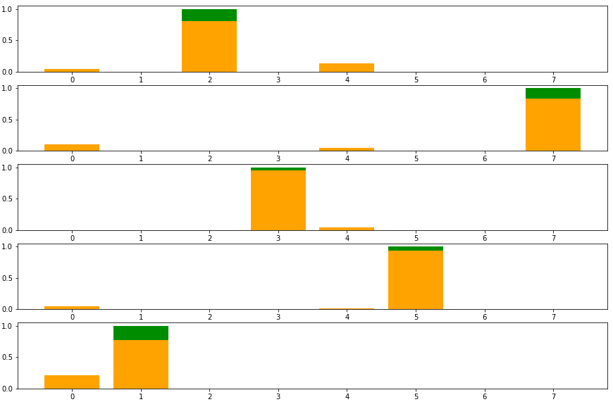
We can see that the network has learned pretty well, most of the green bars are filled with orange. Actually, if we let the training continue for several more epochs, there would be hardly any green on the plot, since the network would have approximated the attention function almost perfectly.
The full code can be accessed here.
From this post, we have witnessed how Attention works and how to train a model to guess the true attention function of the data. I hope this serves as a good starting point for your journey into the very interesting miracles around these Attention mechanisms.
Happy learning!
Reference: