Batch Normalization and why it works

Test your knowledge

Batch Normalization (BatchNorm) is a very frequently used technique in Deep Learning due to its power to not only enhance model performance but also reduce training time. However, the reason why it works remains a mystery to most of us. Furthermore, many tutorials and explanations on the Internet interpret it ambiguously, leaving readers with a false perception of the problem.

In this article, we attempt to give an introduction to BatchNorm, including what it is and why it works in the objective and up-to-date point of view.

Batch Normalization

BatchNorm was first proposed by Sergey and Christian in 2015. In their paper, the authors stated:

Batch Normalization allows us to use much higher learning rates and be less careful about initialization. It also acts as a regularizer, in some cases eliminating the need for Dropout.

which was then verified by many other researchers, building the popularity of BatchNorm.

Batch?

Deep Neural Networks are trained with Gradient Descent optimization, most commonly, the Stochastic Gradient Descent variant.

With Gradient Descent, the process operates in steps, with each step involves feeding data to the network. There are 3 standard strategies of inputting data:

Input one random data point. This is known as the original SGD.
Input all data points. This is the original Batch Gradient Descent.
Input a random mini-batch of date points. Its name is Mini-Batch SGD.

To date, the Mini-Batch SGD is preferred in the Deep Learning community as it has some advantages over the other two:

It is faster than the original SGD since processing m data points at once is less time-consuming than m times of working with one point.
Its gradient updates are less noisy than the original SGD.
It has a higher chance of escaping from local minima than the Batch Gradient Descent.
It is more flexible as the batch-size can vary.

Normalization?

Normalization is the process of bringing values to a standard form.

In the scope of Machine Learning, normalization often means returning the values to a distribution of 0-mean and unit variance.

Batch Normalization?

Batch Normalization is the act of applying normalizations to each batch of the Mini-Batch SGD. These normalizations are NOT just applied before giving the data to the network but may be applied at many layers of the network.

For a layer with d-dimensional input $x = (x^{(1)} ... x^{(d)})$ , we apply normalization to each of the dimension separately. In other words, $x^{(k)}$ is transformed independently from other dimensions. For readability, from now on, we will omit the $(k)$ in the nomination of $x^{(k)}$ .

Given that the input is a vector of size m ( $x_{1...m}$ ), with $m$ being the batch size. The BatchNorm is described as below:

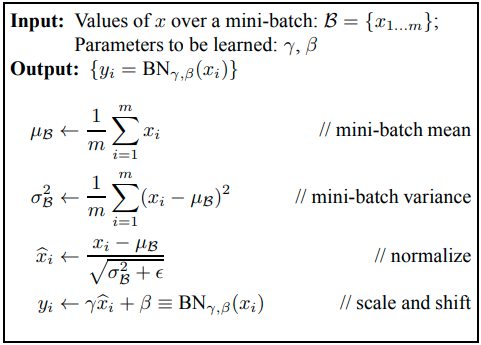
BatchNorm algorithm — The transformation of BatchNorm, taken from its original paper.

where:

$\gamma$ and $\beta$ are 2 additional parameters for each dimension of the input. They are also learned along with the other parameters in the Back Propagation process. $\gamma$ and $\beta$ , as outlined by the authors, attempt to restore the representation power of the networks, since simply transforming input data to a 0-mean unit-variance distribution may change what the layer represents (e.g. in Sigmoid nonlinearity, this transformation may limit the output to the linear regime).
$\epsilon$ is a small constant added for the numerical stability of the computation (i.e. cases when $\sigma_B$ equals 0).

The authors suggested that BatchNorm may be used either immediate-before or immediate-after the activation functions. In their experiments, BatchNorm is added right-before the nonlinearities. However, some other researchers found using BatchNorm after nonlinearities can produce better outputs. The same test even indicates that removing the scale-and-shift phase (using $\gamma$ and $\beta$ ) may increase the model’s performance.

The benefits of using BatchNorm

As described in the paper, BatchNorm helps in both speed and accuracy. To be more specific, it:

reduces the dependence of gradients on the scale of the parameters or of their initial values. This allows us to use much higher learning rates.
introduces noises to the data, hence acting as a regularizer, in some cases eliminating the need for Dropout. This noise introduction comes from (1) the act of transformation itself and (2) the means and variances of different mini-batches might vary slightly.
ensures that the distribution of nonlinearity inputs remains more stable as the network trains, then the optimizer would be less likely to get stuck in the saturated regime. Thus, this enables the uses of saturating nonlinearities (e.g. Sigmoid and Tanh) and relieves us from careful parameter initialization.

Even though the effectiveness of BatchNorm is inarguable, some of the reasoning from the authors is not agreed by many other researchers. We will elaborate on this in the subsequent sections.

Good practices with BatchNorm

Increase the learning rate. BatchNorm allows higher learning rates to fasten training without breaking out the model.
Remove or reduce other regularization methods. As BatchNorm already regularizes the model, the need for further regularization (e.g. Dropout, adding noise) is lessened. This point is affirmed by separate experiments here and here.
Accelerating the learning rate decay. As the model is training faster, the learning rate should also decay sharper.
Shuffle training observations more efficiently. There should not be some observations that always appear in the same batches together, as this could make the transformation of BatchNorm more definitive, which in turn reduces the regularization effects.

Test your understanding

Why does BatchNorm work?

The authors’ reasoning

Back Propagation (BackProp) is a powerful technique to train Neural Networks, however, it has the disadvantage of assuming all the previous layers are fixed when updating each specific layer. Put it differently, at each backward step, BackProp updates all layers simultaneously, moreover, the updating value of layer i-th assumes all previous layers (all layer j-th, with j < i), are fixed, which is not true as all the network is changing. The continuous change in the distribution of each layer’s input is called the Internal covariate shift (ICS).

While this assumption simplifies the learning problem and makes the BackProp works, it is always violated, making the optimization process sub-optimal.

A solution to this problem is to decrease the learning rate, which lessens the changes in weights, which, in turn, makes the assumption more valid. Nonetheless, small learning rates diminish the speed of training, thus do not contribute any good to the process.

Another means is to be careful with parameter initialization, which is the direction taken by many previous studies.

Batch Normalization is introduced to partly solve this problem. It “standardize” the input of each layer in term of mean and variance in order to keep the ICS low.

In short, it is mainly:

BatchNorm $\underrightarrow{\text{makes}}$ Low ICS $\underrightarrow{\text{makes}}$ efficient learning

A side-effect that also turned out to be good is that the noise generated through the process helps with regularization, enhancing the generalization ability of the networks.

The explanation of reducing ICS, however, is not concrete as there are some questions still remain unanswered:

Is restraining only the mean and variance enough to ensure the low ICS, while other characteristics of the input are free to change?
Since $\gamma$ and $\beta$ are altered at each training step, the mean and variance of the input would also vary, so how do they keep the ICS low?
should there be more empirical proofs of the causation of low ICS to more efficient training?

Researches are conducted to answer the above questions. For example, this paper from Johan et al. argues the success of BatchNorm can be explained without ICS.

Ian Goodfellow’s lecture

Ian Goodfellow is the creator of GAN (Generative Adversarial Network), author of Deep Learning Book, and is also one of the pioneers of Deep Learning.

In his lecture on Batch Normalization, Ian stated his view on the reason why it works: because $\gamma$ and $\beta$ help control the higher-order statistics.

As the Gradient Descent algorithm uses only first-order statistics to compute the optimization updates, we are unable to track the higher-order terms, which becomes increasingly important as the networks getting deeper. A change in the weights of one layer does not only influence the immediate successive layer but also the further layers on the net. (This matter is already well-known in the community of Deep Learning. )

Alternatively, the effects of higher-order derivation can be thought of from the secondary-school-Physics point of view. In Physics, the velocity is the derivative of position, while the acceleration is the derivative of velocity (or says, acceleration is the second-order derivative of position). By knowing velocity, we can somehow estimate the value of the position after an amount of time. Nonetheless, if the amount of time is large, the acceleration may change the velocity in the meantime, making our estimation further inaccurate. Hence, we are forced to set a small time frame. In this example, the position is analogous for the weights, velocity for the first derivative, the time frame for the learning rate, and acceleration for the higher-order derivatives. As we only know the first derivative (velocity), we have to set a small learning rate (time frame) in order to have an accurate estimation without being affected too much by the higher-order derivatives (acceleration).

According to Ian, by using BatchNorm, the statistics of a layer are controlled by only two parameters $\gamma$ and $\beta$ , which is much easier for the subsequent layers to adapt to, instead of all the complex sets of weights. Furthermore, by letting these 2 parameters be learned, the original distribution of the input can be recovered if necessary.

Ian’s point of view, although not related to ICS, still mostly agrees with the authors of BatchNorm.

However, this interpretation remains a hypothesis without solid evidence. The above-mentioned experiment from Ducha-Aiki is, in one way or another, opposite to Ian’s thought when showing that BatchNorm without $\gamma$ and $\beta$ gives a stronger performance over the conventional one in his case.

Shibani et al.’s view

Shibani et al. published a paper with the name being literally “How Does Batch Normalization Help Optimization?“.

In their research, they suggested 4 crucial points:

While the network does attain better performance with BatchNorm, the use of BatchNorm in fact often increases the ICS, which contradicts common knowledge. Furthermore, in the case of Deep Linear Networks, the standard network experiences almost no ICS for the entire training, on the other hand, for the network with BatchNorm, the difference in gradients before and after updates is high (which is contrary to the normal understanding that BatchNorm reduces ICS, which in turn makes the gradients change lesser).
ICS has little (or none) to do with the performance enhancement given by BatchNorm. In the experiment, they added time-varying, non-zero mean and non-unit variance noise independently after each BatchNorm layer in order to purposely increase the ICS. The resulting noisy-BatchNorm-network exhibits higher performance than the standard network without BatchNorm and closely matches the no-noise BatchNorm network.
Moreover, the same process of adding noise, when being added to the non-BatchNorm standard network, prevents it from training entirely.
The key impact that BatchNorm has on the training process, as they stated, is to reparameterize the underlying optimization problem to make its landscape significantly more smooth. To be more specific, it improves the Lipschitzness of the loss function and also makes gradients of the loss more Lipschitz. These effects ensure more reliable and predictive gradients, enabling the use of larger learning rates and lower the sensitivity to hyperparameter choices.
On a side note, for a constant L, a function f is L-Lipschitz if $| f(x) - f(y)| \leq L|x - y|$ for $\forall x$ $\forall y$ . Function f is $\beta$ -Lipschitz if $|\nabla f(x) - \nabla f(y)| \leq \beta |x - y|$ for $\forall x$ $\forall y$ . (More characteristics of $\beta$ -Lipschitz can be found on the lecture notes from Rutgers university here and here.)
The authors’ mathematical proof of the above statement is presented in their paper.
The standard normalization strategies ( $\ell_p$ ) also give the same performance as BatchNorm. From the paper:

“We study schemes that fix the first-order moment of the activations, as BatchNorm does, and then normalizes them by the average of their $\ell_p$ -norm (before shifting the mean), for p = 1, 2, ∞.”

and

“We observe that all the normalization strategies offer comparable performance to BatchNorm.”

On a side note regarding the normalization schemes, this paper from Elad et al. also provides an interesting insight (although not so related to our topic).

Conclusion

In this article, we have a discussion of Batch Normalization, what it is, how it works and the reasons that make up its reputation.

Sergey Ioffe and Christian Szegedy, the authors of BatchNorm, proposed a wonderful technique to boost both the performance and speed of Deep Neural Networks. However, as concurred by the majority, their reasoning about the work is obscure, leaving a lot of confusion and disagreements.

Recently, there are a number of researches attempting to demystify the mystery behind BatchNorm. One of them is from Shibani et al., who conducted an in-depth experiment, proving that ICS is un-correlated with BatchNorm’s success. Furthermore, they figured out the root cause that makes BatchNorm work, which is mainly from its ability to smoothen the optimization landscape by making the gradients of the loss more Lipschitz. To date, this seems to be the most plausible explanation provided being backed up by experiments and mathematical proofs.

References:

Batch Normalization original paper: link
A test of BatchNorm by Ducha-Aiki on Github: link
Xiang Li et al.’s paper about Dropout and BatchNorm: link
Ian Goodfellow’s lecture on BatchNorm: link
Shibani et al.’s paper about how BatchNorm helps: link, discussion: link
Johan et al.’s paper about Understanding BatchNorm: link
Mlexplained’s post about BatchNorm: link
Paperspace’s post about BatchNorm: link
Rutgers university’s lecture on Lipschitz continuity: link and link
Elad et al.’s paper about Norm in deep networks: link

Tung M Phung's Blog

Batch Normalization and why it works

Leave a ReplyCancel reply