Imbalanced Learning: sampling techniques

How to deal with imbalanced datasets is a traditional but still everlasting problem in data mining. Most standard machine learning algorithms assume a balanced class distribution or an equal misclassification cost. As a result, their performance for predicting uneven data might get doomed by the various difficulties imbalanced classes may bring up.

In this article, we will first give the definition and state some common knowledge of the imbalanced-data problem. Then, a number of sampling methods are explained as potential solutions. We also show the experimental results collected from highly-appreciated papers proposed by experienced researchers in the field.

Test your knowledge

Imbalanced learning introduction

In classification, the imbalanced problem emerges when the distribution of data labels (classes) is not uniform. For example, in fraud detection, the number of positive data points is usually overwhelmed by the negative points. The ratio of different classes might be 1:2, 1:10, or even more extreme than 1:1000 in some cases. Strictly speaking, any ratio other than 1:1 is a sign of imbalance. However, we often attempt to fix the class distribution only when the difference is higher than a threshold, with the threshold value dependent on each specific dataset and user’s purpose.

Types of imbalance

With regard to where it occurs, there are Between-class and Within-class imbalances.

The Between-class imbalance is more common and easier visible to our eyes. It indicates that the numbers of instants for different classes are not comparable. For example, a dataset with 10k Positive samples and 50k Negative samples suffers from this problem as their between-class ratio is 1:5.
The idea of within-class imbalance is more subtle. It implies that different subconcepts of the same class have different numbers of supporting data points. What is a subconcept? It is like a cluster of similar points, a subconcept of a class represents a local space so that all the data points inside the space belong to the same class. One class may have multiple subconcepts. For example, suppose we have a dataset of companies in which the label is a binary value indicating if the company is operating well in the coronavirus-time (Positive) or not (Negative). Inside the positive class, we may have 20 big, prestigious, and sell-with-cheap-price e-commerce companies (subconcept 1) and 100 medical mask-producing companies(subconcept 2). These 2 subconcepts are completely separated and their numbers of instants are not equal, causing the within-class imbalance problem.

Demonstration of between-class and within-class imbalance. — a) Between-class imbalance: The circle class has many more data points than the star class. b) Within-class imbalance: one class may contain multiple subconcepts (e.g. the star class contains white star and black star subconcepts) and the number of examples from each concept is different. Figure from this paper.

With regard to the nature of the problem, there are Intrinsic and Extrinsic imbalances.

The Intrinsic imbalance refers to the cases where the dissimilarity of data sizes is real not only in our dataset but also in nature. In other words, it means that our dataset reflects the population well, and the imbalance in our dataset is caused by the imbalance in the population.
The Extrinsic imbalance, on the other hand, says that the actual population data is not the issue, but our dataset does not represent the population well and that is the reason for the imbalance. For example, the population contains roundly 50% of each Positive/Negative data, yet, due to some bad designs and mistakes during the data collection phase, our dataset contains sample data with the class ratio of 1:2. That is called Extrinsic imbalance.

With regard to the minority class’s size, there are Relative and Rare instances imbalances.

The Relative imbalance refers to the cases where the ratio of the minority and the majority classes is unchanged regardless of our data size. For example, suppose our data is now consisting of 1k minority-class and 9k majority-class data points. If we try to collect more data, say, to increase the size to 100k in total, the expected number of corresponding data in minority and majority classes are 10k and 90k, respectively.
The Rare instances imbalance, on the contrary, tells that regardless of how we expand our dataset, the number of minority-class samples cannot increase. Let’s take cyber-security as an example. Suppose we have a collection of connections to your company’s servers and each of the connections is marked as malicious (say, a hacker uses that connection to steal your company’s data) or not. Here, the positive data points are the ones that were detected by the security team in the past. All the positive data points we can possibly have are already in our dataset and we cannot add more of them by collecting more, older connections.

It is important to note that some studies suggested that the relative ratio of the minority class might be unharmful to the model predictions in some cases. In their paper, Weiss and Provost stated that:

…as more data becomes available, the choice of marginal class distribution becomes less and less important…

They emphasized the importance of the absolute number of minority-class data points: when the minority class is big enough, the relative imbalance will cause less damage to the classification model. However, be cautious that their metrics of performance measurement were Accuracy and AUC (Area Under the ROC Curve), and these metrics are later argued as unsuitable for imbalanced learning problems (here, for example).

More generally, in this paper, Japkowicz and Stephen concluded that the problem of imbalance data is worsened with:

…the higher the degree of class imbalance, the higher the complexity of the concept, and the smaller the overall size of the training set…

Common assumptions

The imbalance may occur in every classification problem. However, in most literature, if not stated clearly, the scope is often assumed to be in binary problems.
Furthermore, the positive class usually represents the minority (thus, the majority is the negative class).
In general, if the False Positive and False Negative costs are equal, we don’t need to handle the consequences of imbalanced data at all. Hence, almost all the time talking about imbalance learning, the 2 types of error have different costs.
Moreover, the minority class (the Positive one) is considered to have a higher misclassification cost than the majority (the Negative class). This complies with most real-world situations when a false prediction of a positive case causes more damage than the other way around (e.g. the detection of malicious internet connection, cancer detection, fraud detection). On the other side, be warned that there are also a few situations when the False Positive cost is much higher, e.g. spam detection.
For the sake of abbreviation, a majority (or minority) class example may sometimes be called a major (or minor) point/data point/example.
The F-value, F-score, and F-measure are synonyms for the same performance measurement metric and can be used interchangeably.

Solutions by Sampling methods

Random over/under-sampling

Random oversampling means we do bootstrap sampling (random with replacement) of the minority class and add it to the dataset. Random oversampling will create multiple duplicated data points.

Advantages

Simple and less time-consuming.
The newly-added data points are all correct because they are copies of the original points. This is in contrast with synthetic oversampling when novel data points are generated by manipulating existing points, thus, the generated point might be not consistent with the real world.
We don’t need to define a distance to measure the difference between each pair of data points. Finding a good distance function is not easy in many cases. This is in contrast with, for example, k-means based methods we describe below.
Despise its simplicity, random oversampling offers competent results in many situations.

Disadvantages

Duplicating a small number of data points (the minority points) might make the model more prone to over-fitting.
Oversampling increases the training size, thus the training time is lengthened.

Random undersampling means we take only a subset of the majority points to train with all the minority samples. By doing undersampling, we reduce the relative imbalance of data by sacrificing a portion of the larger class(es).

Advantages

Simple and less time-consuming.
There are no artificially-created data points added to the dataset. Thus, there is no chance of falsifying the data samples.
No need of defining a distance function for pairs of data instances.
Model-training time might be reduced due to the smaller dataset.

Disadvantages

The biggest drawback of undersampling is the risk of losing information from removing data points. For example, if the original class ratio is 1:9 (i.e. the majority class is 9 times bigger than the minority), to make them comparable in size, i.e. 1:1, we would need to exclude 80% of the data.

Different studies have different views of over and undersampling performance. As an example, in this paper, Batista et al. concluded that when using C4.5 as the classifier, oversampling outperforms undersampling techniques. However, also using C4.5, Drummond and Holte found that undersampling tends to be better than oversampling.

Nevertheless, in some research, the strength of random over/under-sampling is even higher than some other more complex techniques. To be more specific, in this text, Yun-Chung stated that:

Regardless, we still feel it is significant that random undersampling often outperforms undersampling techniques. This is consistent with past studies that have shown it is very difficult to outperform random undersampling with more sophisticated undersampling techniques.

Ensemble-based sampling

EasyEnsemble

The EasyEnsemble method independently bootstraps some subsets of the majority class. Each of these subsets is supposedly equal in size to the minority class. Then, a classifier is trained on each combination of the minority data and a subset of the majority data. The final result is then the aggregation of all classifiers.

BalanceCascade

If the EasyEnsemble is somewhat similar to the bagging of weak learners, the BalanceCascade is, on the other side, seemingly related to a boosting scheme. BalanceCascade also creates a bunch of classifiers, the difference is that the input for the subsequent classifiers is dependent on the prediction of the previous ones. More specifically, if a majority-class example has already been classified correctly in the preceding phase, it is excluded from the bootstrap in the successive phases.

The authors of these 2 methods have then published a complementing paper to extensively assess their performance (using AUC, G-mean, and F-score) on various datasets. They conducted an experiment on 16 datasets using 15 different learning algorithms. The result reported is quite promising:

For problems where class-imbalance learning methods really help, both EasyEnsemble and BalanceCascade have higher AUC, F-measure, and G-mean than almost all other compared methods and the former is superior to the latter. However, since BalanceCascade removes correctly classified majority class examples in each iteration, it will be more efficient on highly imbalanced data sets.

As a side note, the classifier the authors used in each training phase of the above 2 methods is an AdaBoost.

k-NN based undersampling

Zhang and Mani proposed 4 k-NN based undersampling methods in this paper. Those are:

NearMiss-1: select only the majority-class examples whose average distance to the three closest minority-class examples is the shortest. This method attempts to take only the majority data points that are at the border of the classes.
NearMiss-2: select only the majority-class examples whose average distance to the three farthest minority-class examples is the shortest.
NearMiss-3: select some majority-class examples that are closest to each minority-class example. This method ensures that every minority data point is surrounded by some majority ones.
MostDistant: select the majority-class examples whose average distances to the three closest minority-class examples are the farthest.

Through experiments explained in the same paper, the performance (in F-score) of these methods are actually not very good. They perform worse or at best comparable to random undersampling.

Cluster-based undersampling

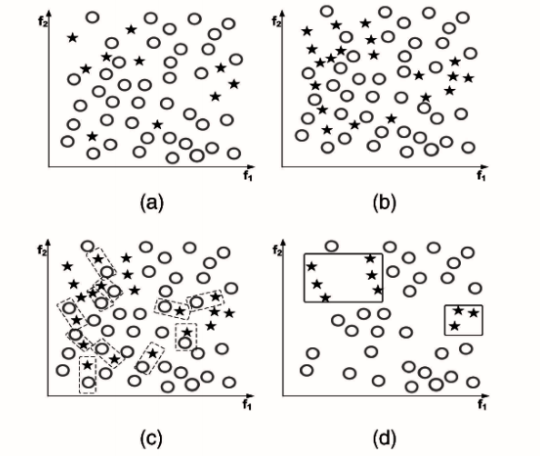
A good observation is that the majority class, which is composed of many data points, might contain many subconcepts. Thus, to obtain a better undersample, we should include data points from all those subconcepts in our selection. We may cluster the majority class, then, for each cluster, a number of data points are selected for undersampling.

This idea is explained in this text by Sobhani et al. To be more specific, they use k-means to cluster the majority examples. After that, 4 methods are experimented to select the representative points from each cluster, including the NearMiss-1, NearMiss-2, and MostDistant methods proposed by Zhang and Mani that we introduced in the above section, together with using the cluster centroids.

There are 8 datasets with different imbalanced ratios (from 1:9 to 1:130) that were used for the experiment. The result, which is measured by F-score and G-mean, shows that clustering with NearMiss-1 performs slightly better than NearMiss-2, while the centroid method is the worst on average. The fact with the cluster centroids is as expected since that method does not include data points at the border, making the model unable to attain a good separation of the classes.

Condensed Nearest Neighbor undersampling (CNN)

The CNN technique also attempts to remove the “easy” data points and keep the ones that are near class borders, yet with a different idea. CNN seeks to find a subset of the original dataset by combining all minority examples with some majority examples so that every example from the original dataset can be correctly classified using the new subset with a 1-nearest neighbor classifier.

To be more clear, CNN finds its subset of choice by:

Initiate a subset with all the minority data points.
For each majority point, try to predict its class with a 1-nearest neighbor classifier on the current subset. If the classification is false, add that point to the current subset.

Note that the above algorithm does not guarantee to form the smallest subset that satisfies the conditions of CNN. We accept this sub-optimal algorithm as trying to find the smallest subset might be unnecessarily time-consuming.

Test your understanding

Synthetic Oversampling (SMOTE)

SMOTE, which was proposed here by Chawla et al., stands for Synthetic Minority Oversampling TEchnique. Unlike random oversampling and the above-mentioned undersampling techniques whose resulting data consists of only the original data points, SMOTE tries to create new, synthetic data based on the initial dataset.

First, SMOTE finds the k nearest neighbors for each of the minority-class data points. Second, for each minor point, it randomly selects one of these k neighbors and randomly generates one point in between the current minority-class example and that neighbor. The second step is repeated until the size of the minority class satisfies our needs.

The SMOTE method is one of the most popular sampling techniques for imbalanced datasets, thanks to its good and stable performance over most types of datasets.

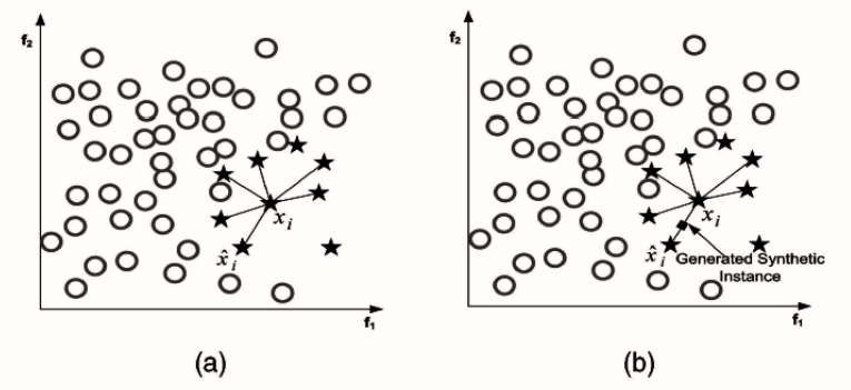
Demonstration of SMOTE method. — Demonstration of SMOTE. a) For each minority data point $x_i$ , k nearest neighbors are taken into account (in this example, we choose k = 6). b) One of the k nearest neighbors is selected at random, then, the new data point is generated randomly between $x_i$ and the selected neighbor. Figure from this paper.

Advantages

SMOTE creates new data points, which solves the problem of data duplication (in contrast with random oversampling). Data duplication often leads to more over-fitting.
It fills the data space, which helps to generalize the dataset.

Disadvantages

There is a chance that the synthetic data points are wrong.
The problem of over-generalization: every minor point generates the same number of synthetic points, which might be not optimal in many cases.

Borderline-SMOTE

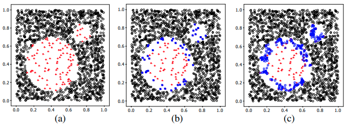
This method is similar to the original SMOTE in terms of trying to generate synthetic minority-class data points from the original dataset. However, for Borderline-SMOTE, only the minor points that are at the border are used as seeds for generating.

To determine whether a minor point is at the border, we consider its m nearest neighbors. If over those m nearest neighbors, the number of major points is at least as large as $\frac{m}{2}$ and smaller than m, this point is considered a borderline minority-class point. Note that if all m nearest neighbors of a minor point belong to the major class, that minor point is considered noise and thus is not chosen.

This method is proposed as a variation of SMOTE that tries to fix its over-generalization problem.

A figure describe how Borderline-SMOTE works in a sample dataset. — The Borderline-SMOTE technique is applied to a sample dataset. a) The original dataset. b) The minority-class data points that are chosen as seeds to generate synthetic data. c) The final dataset after being oversampled. Figure from the original paper.

The authors also did some experiments to compare Borderline-SMOTE with the existing methods (using F-value and True Positive Rate). Over the 4 datasets that were tested on, Borderline-SMOTE and SMOTE show comparable results for 3 datasets, but for the last one, Borderline-SMOTE beats all others for a large margin. It is also worth it to note that the original data without any kind of sampling gives a much worse outcome than with any of the tested methods.

ADA-SYN

Being similar to Borderline-SMOTE, ADA-SYN (adaptive synthetic oversampling) also comes in to address the over-generalization problem of the original SMOTE. However, instead of using a hard cut-off threshold at $\frac{m}{2}$ , ADA-SYN generates more synthetic data points from the minority examples that are surrounded by more majority examples.

In particular, first, a number of m nearest neighbors are identified for each minority point. Then, each minority point $x_i$ is assigned with a ratio:

$p_i = \frac{\Delta_i/m}{Z}$

with $\Delta_i$ is the number of majority points in the m nearest neighbors of $x_i$ , Z is a normalization constant so that $\sum p_i = 1$ . Finally, the number of synthetic points generated from the seed $x_i$ is linearly proportional to $p_i$ .

ADA-SYN can be viewed as a generalization of Borderline-SMOTE with regard to its flexibility. It places more emphasis on the points near the borders but doesn’t abandon the points that are a bit farther away. Furthermore, in the last step, instead of using a linear proportion, we can flexibly change it to a log, a quadratic, or an exponential proportion as needed.

In their experiment with 5 datasets, the authors compare ADA-SYN with the original SMOTE and the original data for a decision tree classifier. It is shown that the G-mean value is highest for ADA-SYN with all datasets, while for F-measure, ADA-SYN is the winner 3 over 5 times. It is also interesting that, as in their experiment, applying a decision tree on the original, imbalanced datasets always results in the best Precision.

Sampling by cleaning

There are 2 crucial reasons behind cleaning:

To remove obvious noise.
To remove data overlapping between classes.

Tomek link

Suppose we have two different data points $x_i$ and $x_j$ , $x_i$ and $x_j$ are of different classes. Let’s call d( $x_i$ , $x_j$ ) the distance between $x_i$ and $x_j$ . If there is no third point $x_k$ such that d( $x_k$ , $x_i$ ) < d( $x_i$ , $x_j$ ) or d( $x_k$ , $x_j$ ) < d( $x_i$ , $x_j$ ), $x_i$ and $x_j$ are said to form a Tomek link. In other words, 2 points form a Tomek link if they are of different classes and each of them is the nearest neighbor of the other.

For a pair of points that form a Tomek link, either one of them is noise or both of them are near a border of the two classes. Thus, we may want to remove all those pairs to make the dataset more concrete and separable.

The trick of Tomek link cleaning is often not performed alone but in companion with a sampling technique. For example, one may remove all Tomek links after oversampling with SMOTE.

Demonstration of applying Tomek-link trick after SMOTE. a) The original dataset. b) The dataset after being oversampled with SMOTE. c) Identify the Tomek links. d) The dataset after removing all Tomek links, which is clearer and more separable. Figure from this paper.

Edited Nearest Neighbor rule (ENN)

The ENN rule seeks to address the same problem as the Tomek link rule, but with a slightly different scheme: A data point is removed if and only if it is different from at least half of its k nearest neighbors, with k is a pre-defined hyperparameter.

Batista et al. did an experiment using Tomek link and ENN together with SMOTE on 13 datasets and showed the result in this paper. The imbalance ratios of these datasets vary from 1:2 to 1:38. Quoted from the paper:

… Smote + Tomek and Smote + ENN are generally ranked among the best for data sets with a small number of positive examples.

Cluster-balancing oversampling (CBO)

The cluster-balancing oversampling technique not only strikes to work on the problem of between-class imbalance but also the within-class imbalance issue. In general, it tries to make the data size of each subconcept more uniform.

The actual behaviors that CBO aims for are:

Each subconcept of the majority class has the same size.
The majority size and minority size are equal (this condition is the same as other oversampling techniques).

To achieve the above, we follow these steps:

Cluster the majority and minority classes separately. They will then have $k_{maj}$ and $k_{min}$ clusters, respectively. Each of these clusters might have its own number of data points.
Let’s call $s_{maj\_max}$ as the size of the largest majority-class cluster. For all other clusters of the majority class, oversample them independently so that each has size $s_{maj\_max}$ . After this step, we have a total of $k_{maj} * s_{maj\_max}$ majority-class data points.
Finally, we oversample each of the minority-class cluster so that each of them has size $\frac{k_{maj} * s_{maj\_max}}{k_{min}}$ .

Note that, unlike the above-mentioned techniques that only oversample the minority class, CBO does oversample both minority and majority classes. The clustering step might be performed using k-means or any other clustering algorithms. Similarly, the oversampling step might also be conducted with random oversampling (as in this paper), SMOTE, or other techniques.

Demonstration of Cluster-balancing oversampling technique. a) The original dataset. The majority class has 3 different subconcepts with sizes 20, 10, and 8. The minority class has 2 different subconcepts with sizes 8 and 5. Each of these subconcepts then forms a cluster. b) The final dataset after CBO. Each majority cluster has a size of 20 while each minority cluster has a size of 30. The size of each cluster belonging to the same class is the same. The size of the minority and the majority classes are equal. The figure is taken and modified from this paper.

Oversampling with boosting

SMOTEBoost

SMOTEBoost was introduced in this paper by Chawla et al. This method integrates SMOTE into each iteration of boosting. That is: before any subsequent weak learner is created, the SMOTE is applied to generate some new synthetic minority examples.

This brings several advantages:

Each successive classifier focuses more on the minority class.
Each classifier is built on a different sampling of data, which helps create more diversity.
Ensemble using boosting helps reduce both bias and variance.

In the same paper, the authors compare the performance of SMOTEBoost with AdaCost, first SMOTE then Boost, and SMOTE only. There are 4 datasets that were used in the experiment. The result is promising: SMOTEBoost, in companion with RIPPER classifier, edges the other methods (on F-value) on 3 over 4 datasets.

DataBoost-IM

Hongyu Guo and Viktor proposed the DataBoost-IM as an adaptation for imbalanced data of their earlier DataBoost, which was aimed to handle balanced datasets. With this implementation, the subsequent classifiers do not only focus on misclassified examples but also give more attention to the minority class.

DataBoost-IM generates synthetic data for both minority and majority classes when maintaining a boosting scheme. In fact, as minority data is usually much harder to learn than the majority data, we expect to see more minority data points on the top of the misclassified ranking, which results in more synthetic minority points generated than majority points.

Let’s call the original training data S, we have $S_{min}$ and $S_{maj}$ are subsets of S that correspond to the minority and majority classes, respectively. At each iteration of boosting, we select m hardest-to-predict data points, call this set E. $E_{min}$ and $E_{maj}$ are the subsets of E containing examples from minority and majority classes, respectively. We expect | $E_{min}$ | > | $E_{maj}$ | since minority points are generally harder to predict. The number of synthetic data points to be generated for the majority class is

$M_{maj} = min(\frac{|S_{maj}|}{|S_{min}|}, |E_{maj}|)$

The number of synthetic data points to be generated for the minority class is

$M_{min} = min(\frac{|S_{maj}| * M_{maj}}{|S_{min}|}, |E_{min}|)$

An experiment with 8 datasets shows that even though the G-mean measurement does not go well with DataBoost-IM all the time, its performance measured by F-score is usually better than other methods, including the aforementioned SMOTEBoost.

Over/Under Sampling with Jittering (JOUS-Boost)

While Random oversampling is easy and fast, it creates duplicates of data (i.e. ties). As having ties potentially makes the classifier more prone to over-fitting, synthetic oversampling techniques like SMOTE are then introduced to resolve this problem. However, these synthetic techniques also have their own drawbacks, they are more complicated and expensive in time and space.

The JOUS-Boost is claimed to be able to address both the weaknesses of the two techniques while inheriting their advantages.

It turns out that, to break the ties, we do not have to move the generated samples to the direction of one of the nearest neighbors, as SMOTE does. Instead, we can move it a little bit to any random direction. This is what is meant by “Jittering”: a little i.i.d noise is added to the data points generated by random oversampling.

Conclusion and further read

The problem of data imbalance might result in a big and bad effect on our predictions and analysis. To deal with imbalanced data, using resampling techniques is a traditional but effective solution.

In this article, we introduce various types of resampling techniques, from simple random over/under-sampling, ensemble-based, k-NN based, cluster-based, SMOTE together with its variants, to combinations of resampling with cleaning, boosting, and jittering.

The reason why there are many resampling techniques of interest is that, according to many studies, none of the techniques is the best for all (or almost all) situations.

…the best resampling technique to use is often dataset dependent…
Yun-Chung Liu, in this paper.

However, overall, we may take it that using ensemble, or to be more specific, boosting, is more beneficial than a single classifier in most cases. Additionally, for each round of boosting, it is recommended to vary some parameters, e.g. the training set and the imbalance ratio.

Other than Resampling, there is another method that is also often used, which is called Cost-Sensitive Learning (the AdaCost we mentioned in the above sections is an example). Furthermore, this alternative method has become increasingly more popular with flying colors:

…various empirical studies have shown that in some application domains, including certain specific imbalanced learning domains, cost-sensitive learning is superior to sampling methods.
Haibo He and Garcia, in this text.

However, it is not so clear who the winner is in dealing with imbalance, sampling, or cost-sensitive techniques. Weiss et al. have conducted an extensive experiment targeting this question and here is their conclusion:

Based on the results from all of the data sets, there is no definitive winner between cost-sensitive learning, oversampling and undersampling.

In general, sampling has its own indisputable advantages:

Not all algorithms’ implementations of cost sensitivity are available.
Some datasets are too big to handle, so undersampling does not only address the imbalanced problem but also makes processing more feasible.

An introduction and discussion about Cost-Sensitive Learning methods for imbalanced datasets will be presented in a future post.

Test your understanding

References:

Learning from Imbalanced Data, Haibo He and Garcia, link
Cost-sensitive boosting for classification of imbalanced data, Y Sun et al., link
The class imbalance problem: A systematic study, Japkowicz and Stephen, link
Learning When Training Data are Costly: The Effect of Class Distribution on Tree Induction, Weiss and Provost, link
The Effect of Oversampling and Undersampling on Classifying Imbalanced Text Datasets, Yun-Chung Liu, link
Cost-Sensitive Learning vs. Sampling: Which is Best for Handling Unbalanced Classes with Unequal Error Costs? , Weiss et al., link
The Relationship Between Precision-Recall and ROC Curves, David and Goadrich, link
Exploratory Undersampling for Class-Imbalance Learning, Xu-Ying Liu et al., link
KNN Approach to Unbalanced DataDistributions: A Case Study Involving Information Extraction, Zhang and Mani, link
Learning from Imbalanced Data Using Ensemble Methods and Cluster-based Undersampling, Sobhani et al., link
SMOTE: Synthetic Minority Over-Sampling Technique, Chawla et al., link
Borderline-SMOTE: A NewOver-Sampling Method in Imbalanced Data Sets Learning, Hui Han et al., link
ADASYN: AdaptiveSynthetic Sampling Approach for Imbalanced Learning, H. He et al., link
A Study of the Behavior of Several Methods for Balancing Machine Learning Training Data, Gustavo et al., link
Class imbalances versus small disjuncts, Taeho Jo and Japkowicz, link
SMOTEBoost: Improving Prediction of the Minority Class inBoosting, Chawla et al., link
Learning from Imbalanced Data Sets with Boosting and Data Generation: The DataBoost-IM Approach, Hongyu Guo and Viktor, link
Boosted Classification Trees and Class Probability/Quantile Estimation, Mease et al., link
Cost-Sensitive Learning vs. Sampling: Which is Best for Handling Unbalanced Classes with Unequal Error Costs? , Weiss et al., link

Tung M Phung's Blog

Imbalanced Learning: sampling techniques

Imbalanced learning introduction

Types of imbalance

Common assumptions

Solutions by Sampling methods

Random over/under-sampling

Advantages

Disadvantages

Advantages

Disadvantages

Ensemble-based sampling

EasyEnsemble

BalanceCascade

k-NN based undersampling

Cluster-based undersampling

Condensed Nearest Neighbor undersampling (CNN)

Synthetic Oversampling (SMOTE)

Advantages

Disadvantages

Borderline-SMOTE

ADA-SYN

Sampling by cleaning

Tomek link

Edited Nearest Neighbor rule (ENN)

Cluster-balancing oversampling (CBO)

Oversampling with boosting

SMOTEBoost

DataBoost-IM

Over/Under Sampling with Jittering (JOUS-Boost)

Conclusion and further read

Leave a ReplyCancel reply