
The Decision Tree is among the most fundamental but widely-used machine learning algorithms. However, one tree alone is usually not the best choice of data practitioners, especially when the model performance is highly regarded. Instead, an ensemble of trees would be of more interest. The ensemble almost always takes in a form of either bagging, random forest, or boosting. Stacking, on the other hand, is often used with multiple types of algorithms.
| Test your knowledge |
|
|
Bagging
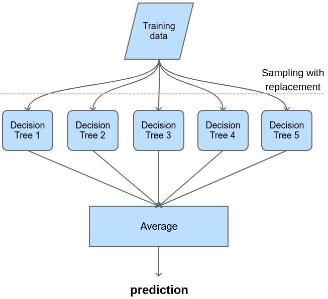
Bagging (Bootstrap aggregating) is the first and most basic type of meta-algorithms for decision trees. Although the concept of bagging can be applied to other algorithms, even a mix of different algorithms, however, it is most commonly used with decision trees. The result outputted from bagging is the average (if the problem is regression) or the most suitable label by the voting scheme (if the problem is classification).
Each decision tree in the bag is trained on an independent subset of the training data. These subsets are random bootstraps of the whole training set. In other words, suppose the training data is a table with n observations on m features. Each component tree of the bagging will receive a subset of k observations on m features to train on, with k < n. Each observation of a subset is drawn from the full data with replacement.
Strengths
The main benefit of bagging is to reduce the variance of the final model while keeping the bias almost uninfluenced. As we already know, the bias-variance trade-off is a perpetual aspect of choosing and tuning machine learning models. Normally, a reduction in the variance always results in an increase in the bias. Bagging successfully makes the bargain to optimize one without sacrificing as much from the other.
How does bagging reduce the variance?
Let’s switch our view from machine learning to basic statistics. Given a distribution with variance  , the variance of 1 data point taken from this distribution is ; the variance of the mean of a sample whose size is s is
  .
.
This property is reflected identically to the space of bagging, where the average of a bag of s independent trees has a variance of , with being the expected variance of each component tree.
What about the bias of the bagging?
Each tree in the bag is trained on a sample of the full training data. Normally, this sample is smaller than the full training data, thus, the bias is increased.
As component trees are identically distributed, the expected bias of each tree is the same, hence, the expected bias of the average of s such trees is also equal to the bias of each tree in the bag.
In conclusion, expectedly, the bias of the bagging model is equal to each component tree and higher than a decision tree model that is trained on the full training dataset.
Weaknesses
Random Forest
Although bagging is the oldest ensemble method, Random Forest is known as the more popular candidate that balances the simplicity of concept (simpler than boosting and stacking, these 2 methods are discussed in the next sections) and performance (better performance than bagging).
Random forest is very similar to bagging: it also consists of many decision trees, each of the trees is assigned with a bootstrap sample of the training data, and the final result of the meta-model is computed as the average or mode of the outputs from the components.
The only difference is that random forests, when splitting a node of a component tree, not all of the features are taken as candidates to split. Instead, only a subset of the whole feature set is selected to be the candidates (the selection is random for each node) and then the best feature from this subset is appointed to be the splitting test at that node. Suppose there are m features overall, the size of the subset can be any number from 1 to m-1, with the most common choices are  and
and  .
.
Strengths
Being similar to bagging, random forests also reduce the variance of the model, thanks to a combination of many trees.
Another advantage of random forests that makes them stand out is the increase of variation of component trees. Because only a small subset of the features is available at each node, the choice of which feature is selected is highly unpredictable, making the trees more different from each other. By virtue of this de-correlation aspect of random forests, the independence of trees gets improved, which results in a stronger effect of variance reduction.
Last but not least, random forests are famous for being a plug-and-play machine learning model. Almost no parameter tuning is needed, which makes it ideal for being a standard, prototype, benchmark, automatic, and versatile model to run everywhere a model is needed.
Weaknesses
As you may have noticed, random forests also inherits the bad sides from bagging:
Extra Tree
Extra Tree (Extremely Randomized Tree) is a variation of Random Forest that worth a separate sub-section to talk about.
Basically, the extra tree scheme is derived from random forests, so they are very close to each other. What make Extra Tree different are:
Strengths and weaknesses
Compared to random forests, the extra tree method is much faster to train, as the heavy work of selecting the optimal cut-point is eliminated. This idea of randomized cut-points also helps with the decorrelation of component trees, with the cost of higher bias. The increase in bias, on the other hand, is somehow relieved by using the full instead of a sample of the training set.
Overall, the performance of random forests and extra trees are pretty close for most problems. On Kaggle competitions, extra trees seem to give a slightly better result in several cases.
| Test your understanding |
|
|
Boosting
While bagging, random forest, and extra tree share a lot in common, boosting is a bit more distant from the mentioned 3 concepts. The general idea of boosting also encompasses building multiple weak learners to contribute to the final result. However, these component trees are built sequentially, one after another, and how to build the latter one is dependent on the result of the formers. Put another way, the next weak learner is built in a way to specifically improve on what the existing weak learners are bad at.
There are a few answers to how should the next tree address the shortcomings of the previous trees, these answers divide boosting into several styles. The most popular styles are Adaboost and Gradient boosting.
Boosting types
Adaboost
With Adaboost (adaptive boosting), the dependency relies on weights. After creating each weak learner, the overall model (so far) is run on the training dataset to give predictions. The residuals of these predictions are then recorded, and samples with higher errors are assigned a higher weight. These weights are perceived by the next weak learner, it will then put more emphasis on the samples that were more inaccurately predicted by the previous learners.
Gradient Boosting
The essential idea of gradient boosting is to build the next learner so that its (the next learner’s) prediction is as highly correlated with the negative gradient of the loss function as possible. The choice of the loss function varies depending on the researcher’s preference. A typical loss function is the L2-error (or squared error), which, after the math, makes the scheme become as simple as the next learner’s target variable is the residual of the last step. (As a side note, the math here is close to that of the OLS, the standard Linear regression algorithm that uses L2 as its lost- or cost – function.)

Strengths
The performance of Boosting ensemble usually surpasses that of Bagging and Random Forest (and Extra Tree). This is empirically proved by the fact that many Kaggle-winning-strategies use Boosting, while the other methods can hardly be found (if any) on the top of the leader boards.
Another advantage of Boosting is that it can perform well even on imbalanced datasets. The fact that there is no voting scheme makes it better in this corner.
Lastly, we can use boosting with an objective function, basically, any function that is differentiable can be accepted. This is profitable because we can optimize our model directly the way we want it to behave.
Weaknesses
While the aforementioned ensembles build independent trees, thus their implementation with parallelization is much easier. For Boosting, the subsequent tree depends on the former ones, which makes the parallelization of trees impossible, resulting in a concern of the high training time. Thankfully, this problem is almost entirely addressed with the parallel inside each tree (i.e. each tree-node is handled by one computer process).
The second issue with Boosting is that it is very sensitive to noise in data and tends to over-fit. In other words, by trying so hard to fit the training data, Boosting models become very low-bias and high variance. There are, in general, 3 approaches to resolve this concern:
- Subsampling: the same technique used in Bagging, Random Forest, and Extra Tree.
- Shrinkage (or learning rate): in Linear regression, the shrinkage of model parameters (e.g. L1, L2-regularization) helps prevent over-fitting. A similar shrinkage can also be applied to Boosting, but what to be shrunk is the effect of the next learners on the entire model.
- Early stopping: as Boosting is an iterative process, early stopping is always a good choice to consider.
The last major problem is with probabilistic output. As stated by Friedman et al. in this paper, boosting (or to be more specific, Adaboost) can be considered as an additive logistic regression model. Thus, it tries to model the output as the logit of the true result, which makes it not suitable to be interpreted as a probability. As an attempt to work out this problem, Mizil and Caruana, in this paper, proposed using Platt Scaling and Isotonic Regression on the outputs to transform them into probabilistic estimations.
Implementations
XGBoost
XGBoost (Extreme Gradient Boosting) is a boosting package developed by Tianqi Chen. Here is a quote from the author:
The name xgboost, though, actually refers to the engineering goal to push the limit of computations resources for boosted tree algorithms. Which is the reason why many people use xgboost. For model, it might be more suitable to be called as regularized gradient boosting.
Tianqi Chen – the original author of XGBoost
The engineering optimization of XGBoost includes (but not limited to):
- Approximation of optimal cut-points.
- The use of sparse matrices with sparse-aware algorithms.
- Parallel computation.
- Built-in regularization.
- Cache utilization.
- Running by GPU.
For the detailed information of XGBoost, you can take a look at its official documentation here.
Around the time it was first invented and published, XGBoost used to be the algorithm-of-choice for Kagglers. Lots of the winners in around the years 2015 and 2016 won their prize using XGBoost.
Light GBM
Light GBM was first released by Microsoft around the end of 2016 with the claim to achieve comparable performance as XGBoost but on a significantly less amount of training time. Empirical experiments do support this claim, many practitioners reported that training a similar model with Light GBM is around 2 to 5 times faster than XGBoost, especially for large datasets.
Light GBM is widely similar to XGBoost in most of its parts. They are almost only different in implementation with some optimizations and heuristics. The fact that Light GBM inherits the idea and some other properties from XGBoost is inarguable. On the flip side, XGBoost also learns from Light GBM for some of its latter updated functions, like the histogram binning option for growing trees. These updates help improve XGBoost’s speed to be almost on par with the other one in some problems.
Overall, these 2 implementations normally output equivalent predictions. Light GBM is considered to be faster than XGBoost and in most cases, is a better choice, at least at the time of writing.
More details about Light GBM can be found on the official documentation here.
CatBoost
Catboost by Yandex is the most recent player in the boosting family. It was first published around the second half of 2017.
As indicated by its name, the CatBoost team seems to put emphasis on handling categorical variables (note that XGBoost only accepts numeric variables). When the data contains a significant number of categorical features, the CatBoost is often expected to outperform the other two competitors, as indicated in this paper by Daoud.
The documentation of CatBoost is here.
XGBoost vs LightGBM vs CatBoost
As always, there is no silver bullet for all problems. Each of the 3 boosting implementations might give a slightly better result than the other two in some cases, both in terms of prediction errors and running time.
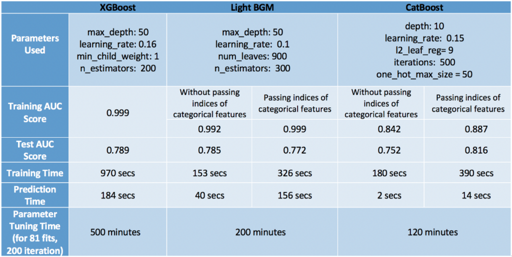
Swalin showed an insightful comparison of them in this medium post. She tested these 3 models on a subset of this Kaggle dataset about flight delays. For this dataset, CatBoost stays on top in terms of accuracy. XGBoost ranked second (with significantly longer running time).
In another comparison by Daoud, the order is flipped: LightGBM showed the best performance while CatBoost is the worst.

Last but not least, in this paper, Anghel et al. show a comparison experiment using 4 different datasets.
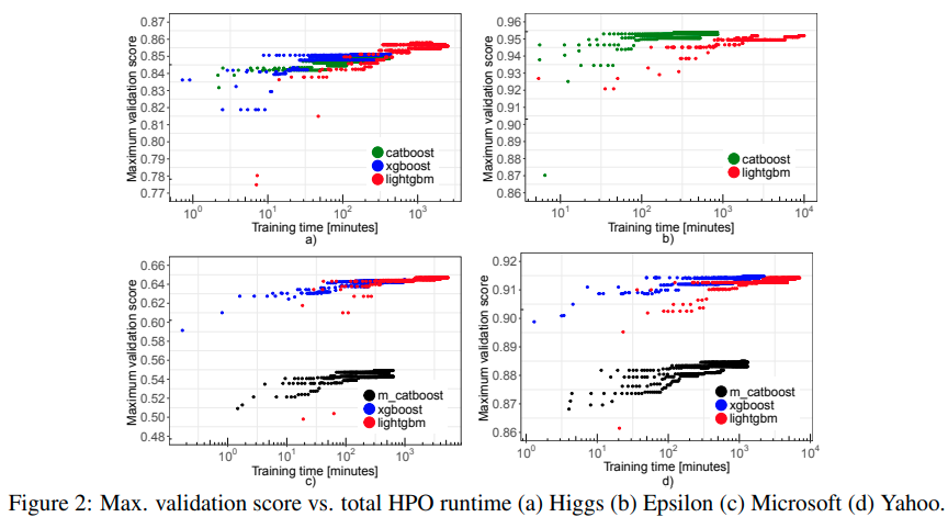
Some highlights are:
- XGBoost cannot process the Epsilon dataset as the input data is too large.
- XGBoost usually finds a meaningful state in a very short amount of time. That is, if your training time is limited to be very short, using XGBoost might be the best choice in general.
- LightGBM seems to be the most stable one. Over the 4 datasets, LightGBM shows reasonable results while XGBoost cannot work on the Epsilon and the performance of the CatBoost on the Microsoft and Yahoo data is substantially low.
As a side note, in the same post, Swalin gives an observation of the parameters of these 3 boosters that worth taking a look:

| Test your understanding |
|
|
Stacking
The last ensemble method we meet in this article is Stacking. Unlike the above-mentioned pals, who often consist of weak learners of the same algorithm (decision tree is the most popular choice for the components), each element of Stacking is usually a different algorithm model.
In other ensembles, each weak learner contributes an additive amount to the final result of the whole. The special approach of Stacking is: each component’s output is considered a feature for the models on the next stack-level to run on. Put it differently, the components of a Stacking are responsible for extracting features.

Strengths and Weaknesses
The use of Stacking is favored in competitions (e.g. on Kaggle) as it can somehow slightly increase model performance in some cases.
However, in practice, it is often regarded as too expensive to use stacking in production:
- The benefit in prediction results is relatively small compared to the big cost of training time and resources.
- Maintenance is more difficult.
- It results in much less interpretability.
Conclusion
In this article, we introduced various ensemble methods that are popular in the world of data science. Bagging is the first and simplest meta-model, which, even though not frequently used these days, is essential to serve as the basis to make the development of subsequent ensembles, like Random Forest and Extra Tree, viable.
Boosting seems to be most regularly used, especially in machine learning competitions. We also distinguished AdaBoost and Gradient Boosting and made acquainted with the 3 most famous implementation of boosting: XGBoost, Light GBM, and CatBoost.
Lastly, Stacking is brought to light with its advantages and disadvantages.
References:
- The Elements of Statistical Learning II, chapter 15: Random Forests, link
- Additive logistic regression: a statistical view of boosting, Friedman et al., link
- Obtaining calibrated probabilities from boosting, Mizil and Caruana, link
- Extremely randomized trees, Geurts et al., link
- Xgboost’s official documentation, link
- lightgbm’s official documentation, link
- Good summary of XGBoost vs CatBoost vs LightGBM, Kaggle, link
- Benchmarking and Optimization of Gradient Boosting Decision Tree Algorithms, Anghel et al., link
- Gradient boosting machines, a tutorial, Natekin, and Knoll, link
- Comparison between XGBoost, LightGBM and CatBoost Using a Home Credit Dataset, Daoud, link
- When would one use Random forests over GBM?, Quora, link
- Differences between stacking, boosting, and bagging, Quora, link
- What are the limitations of linear stacking (ensemble)?, Quora, link
- xgboost: a concise technical overview, Kdnuggets, link
- gbm vs xgboost key differences?, StackExchange, link