
| Test your knowledge |
|
|
Although being used intensively in many applications, from feature engineering to data compression, from tabular to image data, the Principal Component Analysis technique (a.k.a PCA) seems to remain vague for many people. Most of the tutorials about this topic are either high-level or contain extensive maths with lots of abbreviations assuming readers’ extensive knowledge base.
This article, thus, was born with the attempt to make PCA crystal clear to anyone who wishes to understand it thoroughly, step-by-step, in both high and low-level concepts.
An overview
The aim of PCA is to summarize the data.
When a dataset is collected, there may be many features that are similar to each other. For example, in the well-known Ames Housing dataset, which collects information of houses to predict their prices, the 2 features GarageArea (size of the garage in square feet) and GarageCars (size of the garage in car capacity) are highly correlated.
This overlapping information makes it inefficient for processing: data occupies more disk and RAM space, the computational time increases, the predictive models are confused (due to multicollinearity). To facilitate this problem, there are 2 methods in general:
PCA follows the latter option. However, it is a bit more complex than just taking the average, instead, it transforms the entire problem space into a smaller-dimensional space. Suppose, originally, our dataset has 30 features, which means the problem space has 30 dimensions, we may use PCA to project it onto a smaller, say, 10 dimensional-space. Each of the 10 dimensions is a distinct linear combination of the original 30.
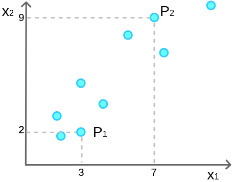
If you feel confused about the above definition, don’t worry. Let’s make it easier using a simpler example. Suppose we have a 2 dimensional-space and we want to reduce it to 1. Look at this figure:

We have 9 samples and 2 features. As you can see, these 2 features ( and
and  ) are highly correlated, when one goes up, the other tends to increase as well.
For the purpose of illustration, let me highlight several random points. Let’s call them P1 and P2, where P1 is in location (3, 2) and P2 is in (7, 9):
Now, as we want to project these 9 points onto a 1 dimensional-space, we should first define what the new space is. This new space may be alone (we just remove from the dataset), or alone (remove ), or a combination of and . What does a combination mean? Well, it is something like g = 0.6 + 0.5 + 0.3. In other words, it is a line in the original space. Let’s make a line g:

We say: g is our new space, we don’t need and anymore, every point is now being measured by the g-dimension only. We discard the 2 old dimensions and project the points on the new dimension:

Yes! We just compressed the data, from 2 features into 1.
At first, our data looks like this:
| Data Point |  |  |
|---|---|---|
| 1 | 3 | 2 |
| 2 | 7 | 9 |
| … | … | … |
Now, it becomes:
| Data Point | g |
|---|---|
| 1 | 1.5 |
| 2 | 6.5 |
| … | … |
Are we done with the PCA? Of course not. We just know that PCA helps us with compressing the features, from d features into k ones, with k  d (in the above, it is from 2 features to 1 feature). We have not learned about how PCA actually does that and proof of its correctness. This will be elaborated in the next sections.
Another example of compressing data is with television. We know we are living in a 3-dimensional world, however, the TV is flat, it can only show 2-dimensional movies. In fact, there are infinite numbers of ways to choose a 2-dimensional basis from a 3-dimensional one (i.e. you can place your eyes in an infinite number of positions). The director (or the cameraman) tries to select the best place to put the camera on, this is analogous to us trying to find the best sub-dimensional space to project the data points so that the most information is retained.
At this point, it is the right time to mention that: everything comes with a cost, as we get the advantage of reducing the dimensionality, we have to trade-off by losing some amount of information from the data, and we try our best to make this loss as small as possible.
Let’s go back to the example above when we have 30 features in our dataset. Suppose we try to apply PCA here, then at the end of the day, PCA gives something like this:
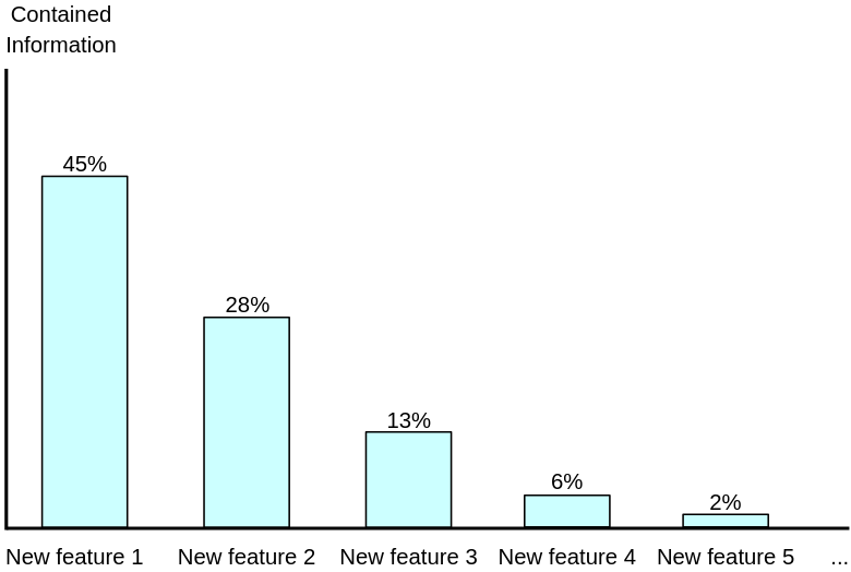
This bar-plot shows how much information we can retain using each new feature. For example, if we compress the original set of features into only 1 feature, 45% of the information is kept; if we compress it into 2 features, 45% + 28% = 73% is kept; if we compress it into 3 features, 86% is kept; for 4 features, the number is 92%, etc.
That said, with using just 4 new features, we manage to keep 92% of the information from the original set of 30 features, which is pretty impressive: the number of features reduced by 86.7% while the loss information is just 8%.
You might have been wondering all along about how information is measured. Information is a vague definition and it is nearly impossible to be measured quantitatively like what we did (45%, 73%, etc.). You are right. What we actually measured here is not really information, but an estimation of information, which is the variance of the data.
Why do we use variance to estimate information? There are several reasons:
Hey, so what are the independent random variables? By independent here, we mean the set of new features has its elements perpendicular to each other (or say, orthogonal). In every sense, they should be orthogonal. Let us elaborate:
Variance
Here we zoom a little bit more into the variance of the data, which is our estimation of the amount of information, about how it is computed.
Look at the example that we have 9 points on a plane and try to compress (or project) the data onto a single line (axis). Projecting these points on the g-axis as follow:
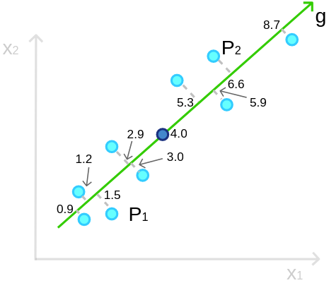
So the values we get are [0.9, 1.2, 1.5, 2.9, 3.0, etc.]. Notice the bold dot at position 4.0, it is the mean ( ) of the 9 points. Then, we compute the variance. The sample variance, as you probably know, is computed by:

In this example,  . That means by using this g-axis, we keep about 7.51 units of the variance of the data.
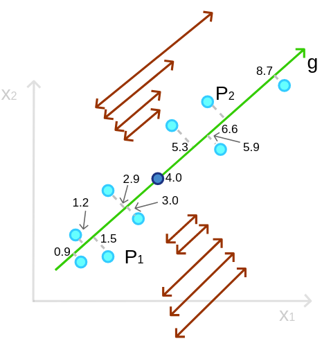
Instead of g, we may choose to use many other axes (in fact, we may choose from an infinite number of axes), for example, g1, g2, and g3 as depicted below.

Each of these axes, when the data points are projected on, gives a different variance. And as we concurred before, we try to find the axis that makes the largest variance, as this indicates the most information from the original data is retained. Just with our eyes, we can say that g2 seems to be a bad choice since the points when being projected on it are condensed in a small range, which causes the variance to be small.
Now again, we come back to the g-axis. If you have ever seen a Linear regression or an OLS, you might tell that the g-axis is kind of similar to a linear regressor that uses to predict (the best-fitted line). That is true, however, they are quite similar but not the same. In PCA, we want to maximize the variance, that is, to maximize the sum (or average) of the squared distances from the mean to all the points:
Interestingly, because the projection is perpendicular, each point forms a right triangle with the mean, and because of the distance between a point and the mean is constant, according to the Pythagorean theorem, maximizing the squared distance between the project-point and the mean is equivalent to minimizing the squared distance between the original point and the project-point:

 is equivalent to minimizing
  . (Pythagorean theorem:
  .)
.)So what does that mean? That means we can say the objective of PCA is to minimize the sum (or average) of the distance between the points and the new axis.
For OLS, assume we use to predict , its objective is to find a linear regressor that minimizes the sum (or average) of the residuals. Look at the visual below, the squares of the grey lines are what PCA and OLS try to minimize.

Interesting, isn’t it?
Ok, we have done with the OLS. Before moving on, let me mention some characteristics of the projections:
| Test your understanding |
|
|
Full explanation
In this section, we will have a thorough view, at a lower level, of PCA and how to conduct it. At first, let us summarize the overview we have had, as well as refreshing some common knowledge we would need in the subsequent proofs.
Summary of the overview
Other prerequisite knowledge
Covariance (matrix)
We already know that the variance is a measure of the variability of a set (or sequence) of values. It depends on the distance from each point to the mean of the set. The formula for variance is:

The covariance, on the other hand, involves 2 sequences of values; its aim is to measure how each of the 2 sequences varies from its mean but with regard to the other sequence.

It is also worth to note that cov(x, y) = cov(y, x), obviously.
People seem to be more familiar with correlation than covariance. These 2 terms are very similar, however, the correlation is more suitable for general usage and comparison since it is unitless. In fact, correlation can be thought of as a standardized covariance, as for any given input, the corresponding correlation is always in the range [-1, 1].
As a side note, the correlation is computed by:

Suppose we have d sequences of values, the covariance matrix for these sequences is a d x d matrix whose element at position [i, j] is the covariance of the i-th and j-th sequence, i.e. cov(sequence. Notice that by this definition, the element at position  , sequence
 )
)[i, i] is the variance of the i-th sequence.
For example, suppose we have 3 sequences: x, y, and z. Their covariance matrix is:

which is also equal to:

Linear transformation (projection)
In Linear algebra, a linear transformation (T) can be represented by a transformation matrix A. While A is a m x n matrix, it maps any points from  to
to  (i.e. from a n-dimensional space to a m-dimensional space). The transformation is done by multiplying A to the left of the point-to-be-projected. That is:
T(x) = Ax
The reason why any linear transformations can be done using a matrix is very simple and direct:
- A linear combination is expressed in the form:
 , with d is the number of dimensions,
  represents the i-th dimension,
  is a sequence of scalars defining the linear transformation.
 - Each row (amongst m rows) of the transformation matrix A acts as a .
For example, suppose we want to transform points from a 3-dimensional space to a 2-dimensional space that has the 2 axes being:  and
and  . The transformation matrix A should be:

If you want to map a point P, e.g. P = [8, 15, -5] to the new space, that would be:

Note that any point P is denoted by the vector that goes from the Origin to P, and a vector is assumed to be in column form ( instead of [ 8 15 -5 ]).
Transpose of a matrix
The transpose of a matrix A (size m x n) is denoted by  (size
(size n x m), which is the flip of A, i.e. [i, j] = A[j, i]. Thus, we say Transpose is a flip operation.

We will also need the property of Transpose on a product:

Eigenvalues and eigenvectors
In linear algebra, we have the definition of eigenvalue and eigenvector.
For a square matrix A, a vector v, and a scalar  , if v is not all-zero and:
Av = v
then v is an eigenvector of the matrix A and is the eigenvalue corresponding to that eigenvector v.
For example:

We say:  is a eigenvector of matrix
  and -4 is the corresponding eigenvalue of this eigenvector. Note that if you scale the eigenvector to whatever amount (e.g.
  ,
,  ), you still get an eigenvector with the same eigenvalue.
Only square matrices have eigenvectors and eigenvalues. Not all square matrices have, however, if a d x d matrix has, it has exactly d pairs of eigenvectors and eigenvalues (except the eigenvectors that are scaled version of some other). These eigenvalues may be distinct or some of them are the same.
For convenience, we also assume all eigenvectors have length 1.
In general, the set of eigenvectors of a matrix are not necessarily orthogonal. Yet, for a symmetric matrix ( ), the eigenvectors are always orthogonal to each other. Prove:
For any real matrix A and 2 vectors x and y, we have:

Suppose x and y are 2 eigenvectors of a symmetric matrix A with 2 corresponding eigenvalues  and
and  , respectively. We have:

Thus  . As
. As  , this means
  = 0, i.e. x and y are orthogonal.
The spectral theorem
According to the spectral theorem, any symmetric matrix is diagonal in its eigenvector basis.
Suppose we have a matrix A with size d x d, A can be written as:

With  …
…  are the orthonormal eigenvectors of A.
If you are looking for proof of this theorem, we suggest Amoeba’s answer on StackExchange, proof by induction on Brilliant, University of Michigan’s proof.
PCA, step-by-step
(Optional) Standardize data
Compute the covariance matrix
Calculate the eigenvalues and eigenvectors
Transform the data
1. (Optional) Standardize data
Suppose we have a dataset (with all numeric variables), the first step is to standardize each feature. Standardization means making each feature have 0-mean and unit variance, i.e.

with being the mean and  being the standard deviation. (The terminology for this is: Z-score transformation.) Amongst these 2 transformations, de-mean is highly-recommended for all cases, while dividing the values for the standard deviation is beneficial in most cases.
a. Why 0-centering?
Basically, in the next step, we will compute the covariance matrix of the data, and as you can see from the formula, 0-centering does NOT have any impact on the values of the covariances. Hence, actually, at least in theory, we do not have to center the data. The reasons we should do it in practice are:
- First, when the means of all variables are 0, the computation of the covariance is simpler, which is:

and the covariance matrix:
b. Why scaling?
The scaling (i.e. dividing by the standard deviation to make it unit variance) should be used when the variables are different on the unit and/or distribution. For example, you have a dataset of companies, 2 of the features are the total asset (assumed to be in the range 0 – 1 billion $) and the number of employees (1 – 10000 people). The former feature has a much wider range of value and its variance is probably much higher than of the latter. This fact makes PCA focuses mainly on the total asset and overlooks the number of employees when it tries to maximize the retained variance of information.
This situation is like when we want to gauss how rich a person is by the number of telephones and the number of houses he has. Person A has 100 phones and 1 house, while Person B has 1 phone and 10 houses. We end up blindly say that Person A is richer than B because 100 + 1 > 1 + 10, which is obviously wrong as the numbers are in different units.
On the other hand, if the features are measured in the same unit and/or of the same distribution, it is advisable to not scale them, as this act may potentially wideout some useful information.
Also, it is good to know that when the variables all have unit variance, the covariance and correlation matrices are equivalent.
2. Compute the covariance matrix
The covariance matrix of the training data is computed using the previously mentioned formula, i.e.:
We re-notice it that some libraries use the simplified formula that assumes data is centered around 0:
If the number of features in the dataset is d, then the size of the covariance matrix is d x d.
Why do we compute the covariance matrix?
Here we reveal a truth: PCA does not find the optimal transformation that maximizes the variance, it is kind of a greedy algorithm, trying to find the best next-axis that maximizes the variance, locally.
That is,
- at first, PCA finds the best vector such that when we project the data points on this vector, the variance of data is the largest, this is the first axis, the first principal component.
- Then, amongst all the vectors that are orthogonal to the first axis, PCA finds the one that maximizes the variance of data when being projected on that vector, this is the second axis, the second principal component.
- Next, PCA selects from all the vectors that are orthogonal to the 2 selected axes, get the one that maximizes the variance, mark it as the third axis, the third principal component, and so on until there are all
dprincipal components (dis the number of data features).
The point here is that PCA is a greedy method, which tries to maximize the local reward at each point of time.
Let’s call X the 0-centered data matrix (size n x d). Now we attempt to find the first principal component, the vector w that maximizes the variance of data when we project on it.
Call X’ the projected data, we have:

This is true because when we want to transform data (X) using a transformation matrix (w), we multiply the transformation matrix on the left of the data (described here). We use the transpose operation to make the operation right. Intuitively, you can observe that when you project data on a 1-dimensional coordinate (w), the resulting point will have only 1 dimension. Here  (size
(size 1 x d) multiplies  (size
(size d x n) gives a 1 x n matrix, which is the values of n data points after being projected. This 1 x n matrix is then transposed too to make the dimension right (we suppose each row is a data point and each column represents a feature).
Using the transpose property, we simplify the equation:

X’ (size n x 1) has mean 0 because  , which, in turn, because X is centered.
Thus, the variance of X’ is:

Or, we can say:

with C being the covariance matrix of the original data matrix X.
Hence, we want to find a vector w, whose length is 1 (why unit length?), such that  is maximal.
That is why we have to find the covariance matrix of the data.
3. Calculate the eigenvalues and eigenvectors of the covariance matrix
Finding the eigenvalues and eigenvectors of a matrix is not a simple task when the size of the matrix is larger than 3 x 3 (you may have known this from your linear algebra course). We are not trying to elaborate on how we do this step ourselves (we can just make use of a library), instead, we attempt to answer the following question as a fundamental part of PCA:
Why do we need the eigenvalues and eigenvectors of the covariance matrix?
As C is symmetric, the spectral theorem tells us that it can be written as  where Q is formed by orthogonal eigenvectors and is the diagonal matrix of eigenvalues. We also sort the eigenvalues (and the corresponding eigenvectors) so that
  .
.
We have:

Because  , it is true that
  since v is nothing more than a transformation of w into a different (but with the same number of dimensions) space using the orthogonal matrix
  .
.
This makes it obvious that the maximum value of  is
is  when v =
  .
.
As  and Q is orthogonal,
  , i.e. w = the vector corresponding to , the largest eigenvalue.
That is the reason why we need to compute the eigenvalues and eigenvectors. Above, we explain the process of finding the first principal component, which turns out to be the eigenvector of the most significant eigenvalue. Looking for the subsequent principal components is almost identical since the fact that we are working on orthogonal space makes finding the next component nearly independent of the previous ones.
To conclude this step, we claim that the variance (as an estimation of information) retained by the principal component i-th is equal to the i-th largest eigenvalue ( ).
).
The below figure, which we had as an example for the overview section, indicates that the first principal component retains 45% of the total variance, the second retains 28%, etc.
It is also equivalent to:


etc.
4. Transform the data
We have gone through the difficult part, the last step is the easy one.
We have an original dataset X (n x d), an orthonormal basis of eigenvectors Q (d x d) with the corresponding diagonal matrix of eigenvalues (d x d), in which the eigenvalues are sorted in decreasing order.

There are 2 general options for transformation:
- We want to reduce the d dimensional data down to a specific k (
 ).
). - We want to reduce the dimensionality as much as possible but at least p % of the variance must be kept. For this, get the smallest number k so that

For either case, we have a specific value of k. Q is the transformation matrix that is supposed to transform our data points (the matrix X) to the new basis (or coordinate) in a lossless way (all variance is kept, but the number of dimensions also remains d). However, as we want the new basis to have only k most-meaningful dimensions, we trim the matrix Q by taking the first k columns of it, call this matrix T.

We transform our data points (matrix X) using this transformation matrix T.

The result we get is a matrix  of size
 n x k, with each data point occupies a row of k features.
| Test your understanding |
|
|
Conclusion
So we are done with the intuition and maths behind the so-called Principal Component Analysis (PCA). Actually, the maths part is more complex than it seems, and we are sure it is normal to have to re-read the article several times in order to fully grasp its content. In case you are still in doubt, you might want to take a look at the reference list or drop me a comment (or message).
As a final note, we want to emphasize that PCA does linear transformations, which means it works best when some of our features are linearly correlated to each other. In case the correlations are not linear, we may try pre-transforming to make them linear before applying PCA. Another option is to use a nonlinear dimensionality reduction method (e.g. Isomap).
Thanks for reading!
References:
- CS229’s lecture note 10 from Andrew NG: link
- Q&A about applying PCA on nonlinear data: link
- Lindsay I Smith’s tutorial on PCA: link
- The nice answers on StackExchange: link, link, and link
- Spectral Theorem explained by University of Michigan: link
- Arturo explains why eigenvectors of a symmetric matrix are orthogonal: link
- Wiki’s page about Transformation matrix: link
- Q&A about centering in PCA: link and link