Reinforcement Learning approaches for the Join Optimization problem in Database: DQ, ReJoin, Neo, RTOS, and Bao

The Join Ordering and Join optimization problems

Join Ordering (or Join Enumeration) is a canonical problem in Database Systems. Given a join query of more than 2 relations, there can be different ways of how we select the order of the joins. Each order of the joins will create a Query Execution Plan (which is a binary tree), and our selection of which order (or which tree) to use can largely impact the cost of operation. Here, cost of operation usually means the time required to execute the plan, however, depending on the user’s interests, it can also refer to other measures, like the memory consumed for execution. Nevertheless, the choice of cost is independent of the content of this article, you are free to assume any cost function you want throughout the article.

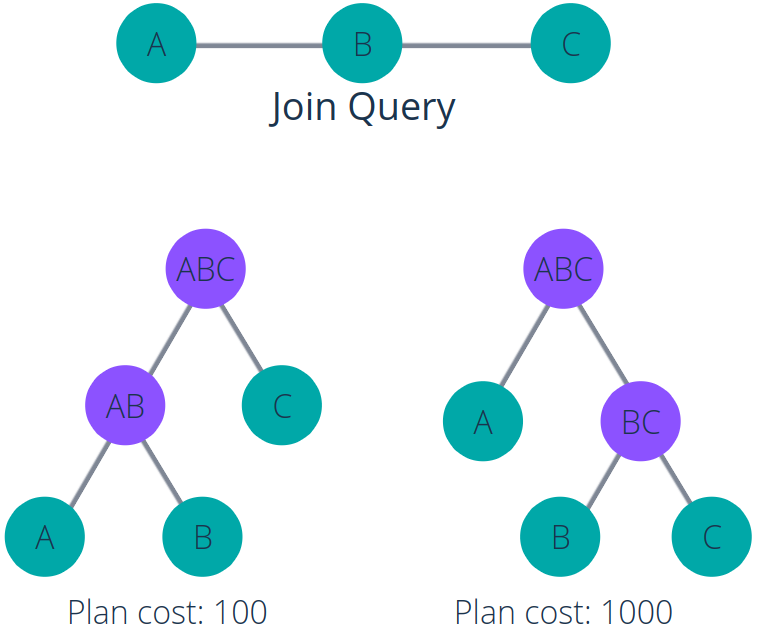
An example of different join orders for a simple query — An exemplar join query and its 2 different Query Execution Plans.

The figure above illustrates a join query and how the join order can affect execute cost. We have a query concerning 3 relations, A, B, and C. It asks for a join between A and B, and a join between B and C.

We have 2 options of how to execute the query. The first option is to join A and B, then take the result to join with C (the tree in the bottom left). The second option is to join B and C, then join A afterward (the tree in the bottom right).

While both options produce the same result, the costs corresponding to these options are different. Here, the first one has a cost of 100, while the second one has a cost of 10 times that much.

In practice, the costs of different plans for the same query can be different in the order of thousands, millions, or even more. Our goal is to find the optimal or nearly optimal execution plan for any given query. Since we can have an exponential number of possible join plans relative to the number of relations, the search space is very large, and finding the optimal plan is actually NP-hard.

The Join Optimization problem is a bit broader than Join Ordering. Besides deciding on the order of the joins, Join Optimization also takes care of some other aspects like the type of the joins (Hash Join, Loop Join, Merge Join).

We need an effective and efficient method to handle this problem. While there are many different approaches, during this work, we focus on the use of Reinforcement Learning (or RL for short).

Reinforcement Learning

Before diving into the details, let us briefly revise some basics of Reinforcement Learning.

The term Reinforcement Learning refers to the umbrella of approaches that try to teach an agent to optimize its action in the environment, while the teaching is done by letting that agent interact with the environment and get the corresponding rewards.

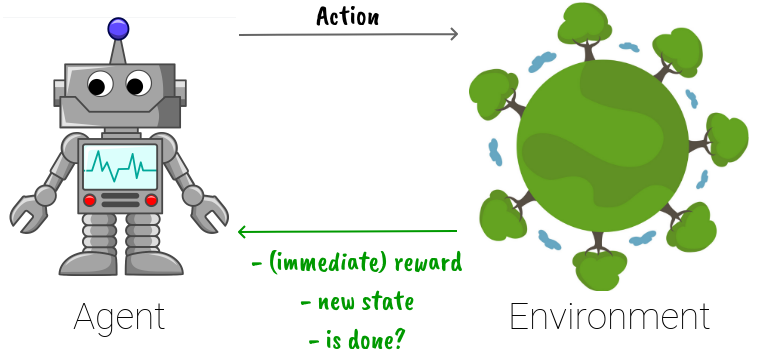
Normally, the agent refers to our computing model, for example, a neural network. The environment can be either a real-life environment or a simulated environment. If you are playing a game, then you or the character you control is the agent, and the whole remaining of the game is the environment. When you take an action, the state changes, you may get an immediate reward and some signals to let you know if your game is done or not (see the figure above). Based on this new information, the agent will take the next action, and so on. The goal is that at the end of the game, the total reward received is maximum.

Some might be confused about RL and AI Planning. They have some similarities, however, they are not entirely the same. Their goals are similar: they both try to find the optimal sequence of actions to go from a starting state to a goal state. Yet, while Planning can freely explore all actions and subsequent states, RL does not have that freedom.

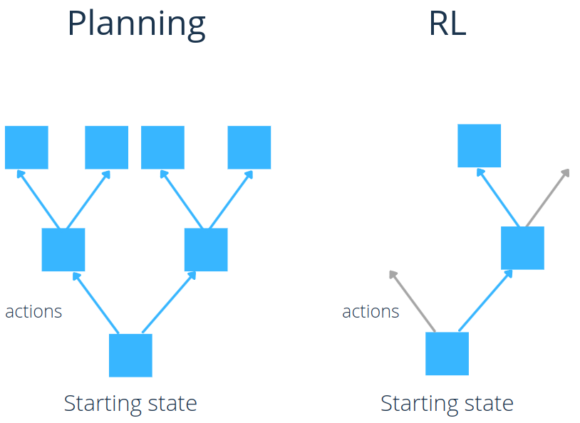
AI Planning vs Reinforcement Learning. A square illustrates a state, while an arrow depicts an action. Blue squares and arrows are the states and actions that the model can try. Grey arrows are the actions the model knows about, but cannot take because, from a state, the RL model can try only 1 action.

With RL in general, from one state, we can take only 1 action. There is no way to, say, try all actions and take the one that produces the best result. That is not possible. In other words, RL is more restricted than Planning, we have less information and we cannot replicate a state.

Reinforcement Learning approaches for Join Optimization

Here, we introduce 5 approaches. The DQ [1] and ReJoin [2] are kinds of the first works in this field. They offer the basic views of how RL can be used for this problem. Neo [3] and RTOS [4] are following works with some improvements. All of them use neural networks as the main computing models. More or less, these 4 models follow the similar structure of having a neural network that inputs the current state of the join and outputs an estimated value (or values) corresponding to taking an action (or each action) in the input state. Their differences lie mainly in how they represent the input (a.k.a featurization) and output, the network architecture, and the training/inferencing scheme.

On the other hand, Bao [5], being the most recent approach, tackles the problem in a completely different way. It doesn’t try to replace the query optimizer but rather complements it.

DQ

In DQ [1], the neural network takes in the query and a pair of subproblems, its output is then a predicted cost value corresponding to joining the 2 subproblems.

To demonstrate how input needs to be encoded before being fed to the neural network, let’s take an exemplar query as below:

SELECT * 
FROM Emp, Pos, Sal
WHERE Emp.rank = Pos.rank AND Pos.code = Sal.code;

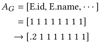
First, we one-hot encode all relation attributes that appear in the query, naming it $A_G$ . Suppose the whole database consists of these 3 relations (i.e. there are no other relations in the database), then all relation attributes are involved in this query.

Next, we encode 2 sub-problems, left and right. The neural network is then trained to answer the question: for this query, what is the cost to join these 2 sub-problems. Suppose we want to estimate the cost of joining Emp and Pos, the encoding of this join should be like this:

where $A_L$ and $A_R$ are the encodings of the left and right sides of the join, respectively.

Finally, the input for the neural network is $A_G \bigoplus A_L \bigoplus A_R$ , where $\bigoplus$ stands for the concatenation operation.

Moreover, it is possible to extend this featurization, for example, with accounts for selection predicates and physical join types.

Suppose we alter the query by adding a selection (Emp.id > 200), as below:

SELECT * 
FROM Emp, Pos, Sal
WHERE Emp.rank = Pos.rank AND Pos.code = Sal.code AND Emp.id > 200;

and further, suppose that the selectivity of this selection is 0.2, then the encoding of the attributes can be changed to below to let the network be aware of this selection:

Attribute encoding with selection predicate

Take a step further, if we enable multiple physical join operators, like Hash Join and Merge Join, we can just concatenate to the featurization an one-hot encoding of the desired join type.

The network is trained with the Q-Learning scheme [6] (refer to this article), a canonical Reinforcement Learning algorithm.

After the network is trained, we can use it to determine the join order by doing the below iteratively until all relations are joined:

At the current state, find all pairs of sub-problems that can be joined to each other.
For each pair of sub-problems, feed it through the neural network to get the estimated cost.
Select the pair with the lowest estimated cost, join this pair.

Main achievement: the authors claim that the average cost of the join plans that DQ outputs is comparable to that from Apache Calcite, PostgreSQL, and SparkSQL.

ReJoin

In ReJoin [2], the network takes in the current state and outputs a heuristic value for each possible join action.

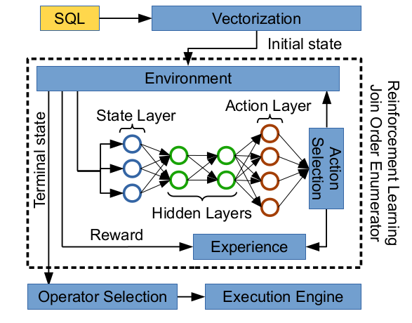
Here, a state consists of the query and the current partial plan. A partial plan is a forest of trees (a tree can consist of a single relation or multiple relations), and we need to join these trees into one, the final execution plan tree. In the beginning, when no join has been performed, we have a forest of trees, where each tree is a singleton.

ReJoin’s neural network outputs a vector, in which each value corresponds to the predicted cost of doing an action. An action here means a join of 2 sub-problems.

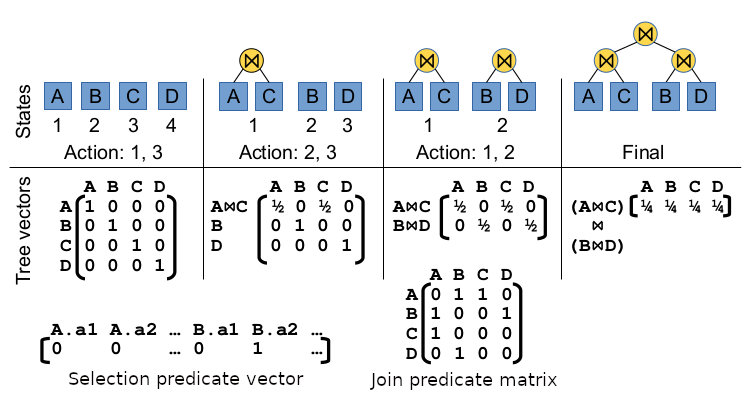
Below, we illustrate the featurization process for ReJoin for an exemplar query:

SELECT *
FROM A, B, C
WHERE A.id = B.id AND A.id = C.id AND B.id = D.id AND B.a2 > 100

Neo's featurization — Input featurization for Neo.

So, what do all of these mean?

The input of the network consists of 3 components: the query’s join predicates, the query’s selection predicates, and the current partial plan.

The join predicates are represented by a matrix of size $N \times N$ , where $N$ is the number of relations in the database. If a join between 2 relations appears in the query, then the corresponding cell in the matrix is 1, all other values are 0.
The selection predicates are represented by a vector of size $M$ , where $M$ is the total number of attributes in all relations in this database. If there is a selection on an attribute, the corresponding value is 1, other values are 0. Note that, in the query above, since the query contains the selection B.a2 > 100, we have a 1 in the Selection predicate vector. We only care if there is a selection on an attribute, but not care what that selection is.
The current partial plan is a forest of trees, in which each tree is either a singleton or a join of multiple relations. The partial plan is represented by a matrix, in which each row represents a tree. In the middle of the figure above, we show 4 different partial plans and their corresponding encodings. Take the second partial plan as an example, the matrix has 3 rows: the first row shows the tree formed by joining A and C, so the values in that row gives 0.5 for A and 0.5 for C. The second row shows the singleton of B, so it distributes 1 to the column corresponding to B.

The input of the network is the concatenation of these 3 encodings above after flattening all matrices into vectors.

The output of the network is a vector of size $N \times N$ , each value represents the cost of joining 2 sub-problems. Note that it is not always that all the values of this output vector are meaningful. Sometimes, the action size is smaller than $N \times N$ . In those cases, we just ignore the invalid positions in the vector.

After the network is trained, we can infer the join tree given a query by iteratively joining 2 sub-problems at a time, the decision to join which sub-problems each time is taken by looking at the output vector (i.e. choose the valid action whose cost is the smallest).

Main achievement: ReJoin outperforms PostgreSQL’s greedy optimizer by 20% in terms of average cost.

Neo

Neo [3] is the updated version of ReJoin with some improvements. The neural network still takes in the current state, which consists of the query and the current partial plan, but only outputs a single scalar as the whole cost of the best final plan that can be constructed from joining the trees in the current partial plan.

We can think of the neural network as a heuristic function that gives a heuristic value for each partial plan. Then, we can use any kind of search algorithms (e.g. A*, Beam search) using these heuristics to find the optimal join plan.

The neural network in Neo makes use of Tree Convolution, a technique to take into account the connection between nodes in partial plan trees for prediction. Tree Convolution and the refined learning scheme help Neo achieve better performance compared to the preceding 2 models with just a small trade-off on planning time (negligible) and complexity.

The neural network architecture of Neo — The neural network in Neo.

The authors also try several methods to encode selection predicates. One method is to use one-hot encoding (as in ReJoin), another is to use selectivity (the same as in DQ). However, both of these are inferior to one that comes from the field of NLP: word2vec. Originally, word2vec uses the co-occurrences of words in the same sentences to induce an embedding for each word in the vocabulary. Here, each row in a relation is analogous to a sentence, and each value in a row is analogous to a word. The idea is to encode each value by a vector so that values that commonly appear in the same context would be encoded by similar vectors. This helps with the encoding of selection predicates.

For example, suppose we have a table Marvel Movies, which has 2 columns Main Character and Weapon, among others. The value “Captain America” of the column Main Character and the value “shield” of the column Weapon usually appear together in the same rows, so these 2 values have similar context and thus, the encodings of selections for these 2 values will be encoded by similar vectors. Suppose, in the training phase, there are lots of queries that have the selection WHERE ... AND Main Character = "Captain America" , the RL model learns a lot about this selection. After that, in the test phase, when the model sees the selection WHERE ... AND Weapon = "shield" then this selection is encoded to a very similar vector as the selection above, which will enable the model to transfer knowledge from the selection above to this selection.

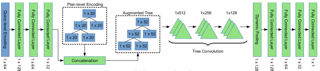
The input to Neo is a concatenation of the query’s encoding and the current partial plan’s encoding. The query’s encoding for an exemplar query is shown in the figure below.

The query encoding is a concatenation of the join predicates’ encoding (i.e. Join Graph in the figure) and the selection predicates’ encoding (i.e. Column Predicates in the figure). Since the Join Graph is symmetric, only the upper half of it (colored red) is used. For Column Predicates, we use the simplest encoding method (a.k.a one-hot encoding) for illustration.

The encoding of the current partial plan is quite unique. A partial plan consists of some trees, and each tree may contain 1 or multiple nodes. The figure below shows an exemplar tree.

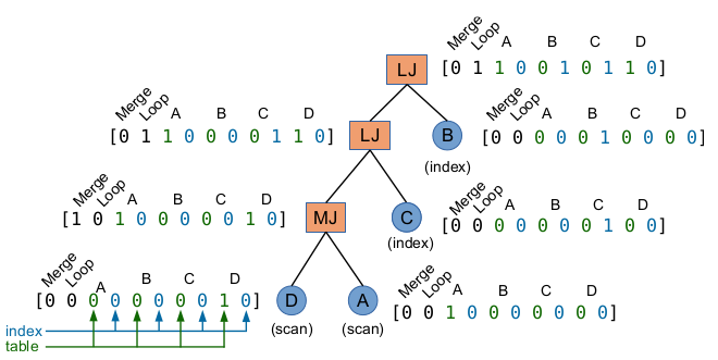
In a tree, each leaf node corresponds to a relation in the database (in the figure, the relations are A, B, C, and D). Each inner refers to a join of its children (MJ is abbreviated for Merge Join, LJ is for Loop Join). Each node is represented by an encoding vector of fixed size, in which the first 2 values are the one-hot of the join type, the green and blue values show what relations are included in the subtree rooted at this node and whether each of these relations is already sorted. Note that this information about sorting is important because, for example, a Merge Join would cost much less if the 2 joining sub-problems are already sorted. The encoding of a tree is then aggregated by applying Max Pooling over its nodes, and the encoding of the whole partial plan is obtained by Max Pooling all its trees.

Main achievement: the performance of Neo is comparable to that of commercial optimizers from Oracle and Microsoft.

RTOS

RTOS [4] is another advanced framework that, similar to Neo, tries to take into account the tree structure and the connection between nodes in partial plans. While Neo does so by using Tree Convolution, RTOS relies on Tree Long-Short Term Memory (or TreeLSTM for short) [7].

How RTOS featurizes the state resembles the other approaches above: concatenating the representation of the query and the current partial plan. In turn, the representation of a query is the concatenation of the representation of its join predicates and the representation of its selection predicates.

We use a matrix of size $N \times N$ to encode the join predicates, where $N$ is the number of tables in the database. This matrix is then flattened to a vector of size $N^2$ . Up to this point, it is the same as in ReJoin. An additional step is to feed this vector through a fully-connected layer, which will give us the representation of the join predicates (see figure below).

Representation of join predicates in RTOS.

The selection predicates for numeric and non-numeric columns are encoded a bit differently. For numeric columns, a selection predicate is represented by a vector of size 4:

$F(c) = (c_{\Join}, c_=, c_>, c_<)$

where $c_{\Join}$ is 1 if this column appears in a join predicate and 0 otherwise; the other 3 values correspond to if the selection operation is =, >, or <. For example, if the selection is WHERE A.x = B.y AND ... AND A.x > 30 and suppose MIN(A.x) = 0 and MAX(A.x) = 100, then the representation of A.x would be (1, 0, 0.3, 0). The first value is 1 because A.x appears in a join predicate. The third value is 0.3 because the selection requires A.x to be larger than 30% from the min value to the max value. The remaining 2 values are 0 because this selection operation is neither = nor <.

For non-numeric columns, the selection operation cannot be > or <. Here, the selectivity of the selection would be put in second place (i.e. the place of $c_=$ ), while the third and fourth places would always be 0.

The representation of a table can then be obtained by applying Average Pooling on its columns.

A partial plan consists of some trees. The figure below shows how we encode a tree:

Look at the bottom of the tree, there are 4 representations, from left to right are the representations of table T1, column T1.a, column T2.a, and table T2, in which T1.a and T2.a are the columns used to join these 2 tables. Then, we apply the N-ary TreeLSTM operation, which outputs the representation of a new table, the one we get by joining T1 and T2. The same process happens in the next step. At this point, we have 2 trees, one combined T1, T2, and T3, while the other one is a singleton of T4. To obtain the representation of the whole partial plan (which consists of these 2 trees), we create a virtual root node on top of these trees, having these trees as its children. The ChildSum TreeLSTM operation is applied on these trees to produce the representation of the whole partial plan. Finally, we concatenate the representation of the partial plan and of the query to get the representation of the current state, which is ready to be fed into the neural network.

Main achievement: the performance of RTOS is better than DQ and ReJoin. If we fine-tune the model with real latency, the result might be even better than the cost-optimal plan generated by Dynamic Programming.

Bao

While all the approaches above attempt to build a learned query optimizer, Bao [5] tackles this problem from a completely different angle. Bao doesn’t act as an optimizer, rather, it sits on top of an existing optimizer and guides it to work better.

Existing query optimizers, like the default one in PostgreSQL, often have the option to let the user forbid themselves to use some of their features. For example, Bao can tell the optimizer to not use Loop joins for a query if it thinks that by doing so, the optimizer will generate a better plan.

We only need to train Bao to correct the existing optimizer rather than create an entirely new optimizer and have it learn from scratch. This reduces the training time enormously.

So what features can Bao forbid the optimizer from using? There are 6 features, 3 of them are join operators (hash join, loop join, merge join), while the other 3 are scan operators (sequential, index, index only). Together, there are $2^6 = 64$ different sets of features, we call them hint sets. Bao’s neural network then selects 1 of these hint sets for each query, and gives its selection to the optimizer to tell the optimizer that it is only allowed to use the operators that are included in the hint set. Note that this network is a value network, it inputs a final join plan and outputs a predicted reward for that plan.

Bao is trained using a modified Thompson sampling scheme, in which, for each input query, Bao tries using multiple hint sets for it, lets the optimizer generate a join plan for each hint set and evaluates the real execution performance for each of those plans. These experiments are then cached to periodically re-train the neural network in the future. An overview of Bao’s architecture is shown in the figure below. In the figure, the neural network is depicted by the 3 triangles with the title TCNN, or Tree-convolution neural network, as Tree Convolution is its essential computing block.

Main achievements:

Bao requires much shorter training time than other Reinforcement Learning approaches.
It is also robust to changes in schema, data, and workload.
Bao has better tail latency, even if compared with commercial optimizers.
Bao works for all types of queries, while other approaches have some restrictions on the types of query (e.g. they all can only handle queries with equi-joins).

Conclusion

Above, we introduced the Join optimization/Join ordering problem in Database together with recent Reinforcement Learning approaches to handle this problem.

DQ and ReJoin are 2 of the first works that started this research direction. However, their performance is already quite encouraging. Neo and RTOS inherit the success of their predecessors and improve upon it. While Neo captures the relationship between nodes in a join tree with Tree Convolution, RTOS tries to achieve the same goal using Tree LSTM. Hand in hand, both of them significantly outperform DQ and ReJoin in terms of performance.

Nevertheless, all these 4 approaches suffer from similar issues. First, they require a long training time. Second, they cannot generalize from one database to another, as well as their inability to adjust to data and workload changes. Third, while their average performance is not bad, occasionally, they generate join trees whose latency is orders of magnitude larger than the optimal ones. Fourth and last, they cannot work for all types of queries (e.g. queries with non-equi-joins, queries with self-joins, or queries with sub-queries).

All these drawbacks are then (at least partially) addressed by Bao, a novel idea that implements a master model that guides the existing optimizer to work better. However, these wins are not without trade-offs. As Bao’s ability is only limited to controlling a set of features, it has limited capability, and thus cannot become much better than the baseline optimizer.

In conclusion, we can see that recently, there are great attempts to apply Reinforcement Learning to the field of Database. While their practicality can be questioned, it is very probable that aspirant researchers can build up from these works and create much better models in the future.

References:

[1] Learning to Optimize Join Queries With Deep Reinforcement Learning, Krishnan, S., Yang, Z., Goldberg, K., Hellerstein, J., & Stoica, I. (2018), paper.
[2] Deep Reinforcement Learning for Join Order Enumeration, Marcus, Ryan, and Olga Papaemmanouil (2018), paper.
[3] Neo: A Learned Query Optimizer, Marcus, R., Negi, P., Mao, H., Zhang, C., Alizadeh, M., Kraska, T., … & Tatbul, N. (2019), paper.
[4] Reinforcement Learning with Tree-LSTM for Join Order Selection, Yu, X., Li, G., Chai, C., & Tang, N. (2020), paper.
[5] Bao: Learning to steer query optimizers, Marcus, R., Negi, P., Mao, H., Tatbul, N., Alizadeh, M., & Kraska, T. (2020), paper.
[6] Q-learning, Christopher J. C. H. Watkins and Peter Dayan (1992).
[7] Improved semantic representations from tree-structured long short-term memory networks, Tai, K. S., Socher, R., & Manning, C. D. (2015), paper.

Tung M Phung's Blog