
In this article, we will discuss the state-of-the-art methods for transforming every kind of input data into fixed-length vectors, including Word2Vec, Doc2Vec, Image2Vec, Node2Vec, Edge2Vec, Code2Vec, and Data2Vec.
Word2Vec
Word2Vec is the umbrella name for all techniques that convert words into vectors.
One-hot encoding
While the simplest method is to represent each word by a one-hot vector, these one-hot encodings do not do well in preserving the relationships between similar as well as opposite words. In one-hot representation, the difference between 2 words that share similar meanings is not distinguishable from a pair of unrelated words. For example, both pairs of words (image, photo) and (image, delicious) have 2 differences in their one-hot encodings, even though the former pair consists of 2 similar words that can be used interchangeably in many cases, while the latter shows 2 completely unassociated words.
Another disadvantage of one-hot encoding is its inefficient use of dimensionality. The vector representation of every word has a length equal to the size of the vocabulary, which can be as large as tens of thousands up to millions in normal situations. This enormous size not only consumes a lot of computer memory but also triggers the various adversities from the curse of dimensionality.
In the next sub-sections, we will introduce great approaches that address these problems. These methods feature words into vectors of a smaller size (from hundreds to several thousand) while preserving the relationship in their meanings (more similar words are represented by more similar vectors).
Continuous Bag-of-words (CBOW) and Skip-gram
Efficient Estimation of Word Representations in Vector Space, Mikolov et al.
Distributed Representations of Words and Phrases and their Compositionality, Mikolov et al.
CBOW and Skip-gram [1] were invented by exploiting 2 key observations:
- Words in a similar context often have similar meanings. Put it differently, similar words tend to appear in similar word neighborhoods. For example, since
imageandphotoare similar, they are often surrounded by the same words, likethis image looks nice,this photo looks nice. But something likethis delicious looks nicenearly never appears in normal corpora. - Neural networks with gradient descent can easily and effectively optimize the vector representation (or embeddings) of words to reflect these similarities in meaning.
Training
Both CBOW and Skip-gram use a neural network as their main computational model. Their architectural differences are shown in the figure below.

CBOW: At first, the sum of the (embeddings of the) neighborhood words is computed. Then, the neural model uses this sum to predict the center word. This method uses multiple (surrounding) words to predict one word (i.e. the center word).
Skip-gram: The neural network uses the (embedding of the) center word to predict the neighborhood words. This method use one word (i.e. the center word) to predict multiple (surrounding) words. Skip-gram showed its superior performance compared to CBOW in most cases and thus, is then re-used in subsequent works that will be presented in this and the following sections.
Experimental results
Note that both methods are self-supervised, meaning they do not require explicit labels from the training data. Nevertheless, the pretrained word embeddings from these models sharply enhance performance in almost all downstream tasks, especially in cases when training data is small or labels are scarce.
Furthermore, since they use networks without non-linear hidden layers, the linear regularities of words are then preserved in their vector representation. For example, vector("King") - vector("Man") + vector("Woman") is most similar to vector("Queen").
An improved version
Putting all these fancy results aside, these 2 methods have a big technical drawback. Be reminded that when the objective is classification, we usually use the Softmax operation on the last layer of the neural networks. Since Softmax is a costly operation (mind the exponentials), having a large number of classes would require a lot of computational power. In this setup, the last layer of the neural network (the classification layer) has a size equal to the vocabulary size (normally tens to hundreds of thousands) and so applying Softmax to all neurons in this layer is not really practical.
In their second paper [2], Mikolov et al. proposed a trick called Negative Sampling to mitigate this issue. The idea is to not apply Softmax to all neurons in the last layer, but only to the positive neurons (i.e. neurons that correspond to the correct classifications) and a random sample of negative neurons. This dramatically reduces the computation while retaining similar effectiveness in training. It is worth it to mention that before Negative Sampling, another trick called Hierarchical Softmax [3] was used for the same purpose. However, Negative Sampling is simpler, easier to implement, and is empirically observed to be better for frequent words and lower-dimensional vectors (though Hierarchical Softmax is better for infrequent words).
Also in the same paper, the author suggested composing phrases out of words prior to training the model. For example, New York should be considered one token instead of a sequence of two tokens New and York. Then, the model will operate on sequences of tokens (a token can be either a word or a phrase) rather than sequences of words as before. How to identify phrases? the frequency of a phrase should be much larger than the product of each word’s frequency alone.
Global Vectors (GloVe)
Glove: Global vectors for word representation, Pennington et al.
GloVe is another approach to represent words by vectors (and is claimed to be better than CBOW and Skip-gram). GloVe shares the same goal with the above 2 methods, which is to learn embeddings of words such that the distances between vectors reflect the differences in the meaning of the words, and that the linear regularities of words are preserved.
Training
GloVe captures the global relationship between words by using a co-occurrence table constructed from the whole training corpus. In simplified terms, GloVe tries to learn the word vectors so that the following equation is satisfied as much as possible:

for all  , where:
 is the embedding of the i-th word in the vocabulary,
 is the dot product of the embeddings corresponding to the i-th and j-th words,
 is the normalized co-occurrence table of words. is a square matrix with
  rows and columns.
  is proportional to the likelihood of observing the j-th word in the context of the i-th word (i.e. the j-th word appears near the i-th word).
This equation makes intuitive sense. If 2 words i and j often appear together, then that means 2 things:
- word
iand wordjhave some relation (or similarity) with each other - is large, or in other words,
 is large. This infers that is also large because the model is optimized to make . Since and
  are kinds of normalized vectors, their dot product is large if and only if they are similar to each other (a.k.a Cosine similarity).
Thus, optimizing for this equation ensures that GloVe embeds similar words by similar vectors.
To go into a bit more detail, GloVe prioritizes optimizing for more-frequent co-occurrences than less-frequent co-occurrences. For example, say AppleiPhone co-occur 1000 times in the corpus, while New and Washington co-occur only 10 times. Then, the model would prioritize making  closer to
  than
than  to
to  .
.
To preserve the linear regularities of words in their embeddings, as in CBOW and Skip-gram, GloVe uses only linear transformations in its computation.
Experimental results
In the demonstrated experimental tasks (i.e. word analogy, named entity recognition, word similarity), GloVe outperforms CBOW and Skip-gram by a noticeable margin.
Fasttext
Enriching Word Vectors with Subword Information, Bojanowski et al.
Fasttext was born to address a problem that previous word embedding techniques ignored: the morphology of words. For example, in German, Tischtennis (which is Table tennis in English) is a combination of Tisch (table) and tennis. This morphology implies that Tischtennis has some relationships with Tisch and tennis, and so it is beneficial to jointly learn their embeddings together. Older embedding techniques did not take this into account and treated the 3 words as completely independent words.
Training
Fasttext handles this issue by representing a word by its character n-grams. The idea is, for each word in the vocabulary, we extract all of its character n-grams (typically, for  ), each n-gram or the entire word is embedded by a vector. Later, the embedding of a word is the sum of embeddings of its n-grams plus the word itself.
With this simple idea, now, representation learning of Tischtennis is intrinsically connected to that of Tisch and tennis as they share some of their n-grams. All n-grams of Tisch and tennis are also n-grams of Tischtennis. Furthermore, some n-grams of Tischtennis, e.g. schten, are not n-grams of the other 2 words, leaving freedom to distinguish their meanings.
For training, Fasttext re-uses the Skip-gram model with Negative Sampling on n-grams (instead of on words as in the original version). Note that despite its name, Fasttext is not necessarily faster than other methods (in fact, the authors reported it to be 1.5 times slower to train than Skip-gram) due to its larger vocabulary.
Experimental results
Regarding performance, Fasttext significantly outperforms the Skip-gram baseline in morphologically rich languages like German, Czech, and Russian. For other less morphologically rich languages like English, the difference to previous methods is not that clear.
Contextual embedding methods
The above approaches try to learn a fixed embedding for each word (or phrase). However, the meaning of a word can be different in different contexts (e.g. bank might mean a financial establishment that allows us to deposit money or the land alongside a river, depending on the surrounding words). Using one embedding for different meanings might result in ambiguities and affect model performance. Contextual embedding methods, thus, learn to embed words concerning their surrounding contexts. A word (e.g. bank) can then be vectorized differently depending on the words around it (e.g. I loan from that <bank> and the river <bank> is nice).
The most renowned contextual embedding model is probably BERT (Bi-directional Encoder Representations from Transformers) [6]. BERT is a large pretrained model on text data. It incorporates the self-attention mechanism to enable the embedding of a word to focus on some other words. For example, take the above sentence the river <bank> is nice, the model can learn to focus on the word river when trying to embed the word bank and thus, it knows exactly the meaning of bank in this sentence.
To dig deeper into how BERT and similar contextual models work, we refer the reader to the original paper [6] and a comprehensive survey of prominent pretrained language models.
Doc2Vec
The ability to vectorize words is great, however, it is not enough for all cases. For example, the task of sentiment analysis requires the model not only to understand the sentiment of words but also how those words as used together to express the sentiment of the whole text.
doc2Vec
Distributed Representations of Sentences and Document, Le and Mikolov
This paper by Le and Mikolov [7] proposed an interesting approach for this purpose. Their model is trained to represent any variable-length piece of text (e.g. phrase, sentence, paragraph, document; from now we will call it paragraph for short) by a dense vector.
Training
There are 2 types of representation for a paragraph, as described below. Each representation results in a dense encoding vector for every paragraph. The final embedding of a paragraph is the concatenation of these 2 vectors.
Representation 1: a distributed memory model of the paragraph.
In this representation, a paragraph is considered a background context such that given this context and a sequence of words extracted from that paragraph, we can predict the next word for this sequence. For example, given a paragraph I think the cat sat on the mat and a sequence of words (the, cat, sat), the model should be able to predict that the next word for this sequence is on. This is illustrated in the figure below.
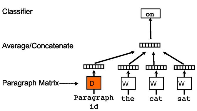
In the beginning, each paragraph is initialized with a random vector. The same happens for each word (i.e. initialized with a random vector). The model takes as input the concatenation of the paragraph vector and a random sequence of word vectors from that paragraph, and is trained with gradient descent to predict the next word. This process repeats for all paragraphs in the training corpus until convergence. In the end, we have a vector representation for each paragraph that serves well as a context for any sequence of words in that paragraph.
Representation 2: distributed Bag-of-words.
In this representation, the paragraph vector is used to predict words in the paragraph without any order (hence the name BOW), as below.
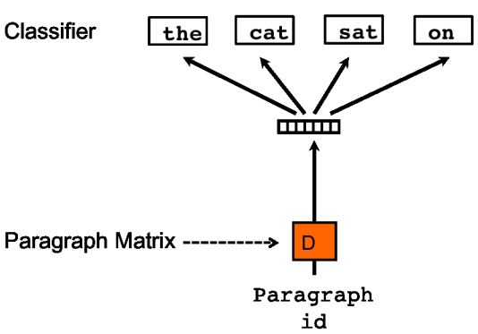
The initialization is the same as in Representation 1: each word/paragraph’s embedding is initialized with a vector of random values. Then, these embeddings are optimized by the model with the objective to predict a random sequence of words in the paragraph without orders (note that this is a multi-label classification problem, in which one input, the paragraph vector, corresponds to multiple labels, the words to be predicted).
After both models for the 2 representations converge, the 2 embeddings for each paragraph are concatenated to form the final embedding of that paragraph.
At inference time (i.e. given a new paragraph, we need to output an embedding for that paragraph), the paragraph vector is inferred by first fixing model parameters and the word vectors, and then training the new paragraph’s vector until convergence.
As an implementation detail, this approach uses a Huffman-tree Hierarchical Softmax to mitigate the problem of using Softmax with many classes.
Experimental results
Experiments show that doc2Vec significantly enhances the performance of the classification model in the tasks of sentiment analysis and information retrieval (i.e. classifying whether a document should be retrieved or not). It not only outperforms baselines like Bag-of-words (which retains no information about the order of words), Bag-of-word-n-gram (which suffers from sparsity), but also more advanced methods like Recursive Neural Networks and Support Vector Machines.
Sentence-BERT
Sentence-BERT: Sentence Embeddings using Siamese BERT-Networks, Reimers and Gurevych
SentenceBERT (or SBERT) is a more recent and more performant approach for embedding pieces of text. Instead of just averaging the BERT output layer or taking the output of the first token (the [CLS] token), which yields lower performance, SentenceBERT attempts to fine-tune the pretrained BERT with a siamese structure to better optimize for the similarities (or differences) between sentences. (Note that while we refer to a piece of text as a sentence, it is equivalent to any variable-length sequence of words, like a phrase, paragraph, or document.)
Training
During the training phase, a siamese structure is constructed with 2 BERT networks (sharing the same weights) as its foundation. This architecture is depicted in the figure below.

Given a dataset in which each instance consists of a pair of texts and a label describing whether the 2 texts are similar, neutral, or opposite, the training architecture tries to predict the label given the input. At first, each input text is fed through BERT to obtain a sequence of embeddings for its tokens, these embeddings are then Mean-pooled to get a fixed-length vector representation for any variable-length text. The 2 fixed-length embeddings for the 2 pieces of text are called u and v. A concatenation of u, v, and |u - v| is then used to classify the label with a Softmax function at the end. Losses are backpropagated to fine-tune the weights of the BERT model in the first blocks.
The total training time for SBERT, according to the author, is less than 20 minutes with a single V100 GPU.
After this training phase, BERT is expected to learn the embeddings of texts more effectively in terms of sentence similarities (or differences). This is true since it was fine-tuned for the task of identifying the relationships between texts.
At inference time, we compute the sentence embeddings of texts similar to computing u and v in the training. Then, these embeddings can be compared with Cosine-similarity (or negative Manhattan, or negative Euclidean distances, whatever similarity measure we like). See the figure below for an illustration.

Experimental results
SBERT is evaluated on the Semantic Textual Similarity (STS) tasks (unsupervised or supervised) and by the SentEval toolkit [24]. In most evaluation datasets, SBERT not only outperforms existing SOTA methods (InferSent [25], Universal Sentence Encoder [26]) but also beat them in terms of inference speed.
The only outlier is with the Argument Facet Similarity corpus with which SBERT underperforms BERT (but this seems to be the case for not just SBERT but all sentence-embedding methods in general).
Image2Vec
Interestingly, while there are multiple works trying to occupy the trending name of <something>2Vec (e.g. Word2Vec, Node2Vec, Edge2Vec), no prominent research papers claimed the term Image2Vec. What are the reasons?
One fundamental reason could be, that, unlike other data types, digital images are already, technically 2-D (greyscale) or 3-D (color) vectors. So, since images are vectors by default, does that mean there is no need for any technique to transform them into vectors? Not really. Words can be easily transformed into one-hot vectors, but as we mentioned, there are many disadvantages to doing so. Similar problems also occur if we use the raw pixels as a representation for images.
Another reason could be that featuring images into fixed-length vectors is a canonical research field that has been actively worked on for a long time (probably from some time in the 20th century), but the trendy <something>2Vec names only started with Word2Vec in 2013. Thus, it does not make sense to rename a long-existed field to follow the new naming style.
That said, even though there are no approaches explicitly named Image2Vec, there are a lot of models that actually do the work. Actually, most of the Deep neural networks for computer vision compress images into vectors before stacking some last layers on top to do downstream tasks like classification or generation. Interesting models include, but are not limited to AlexNet [9], VGG [10], ResNet [11], EfficientNet [12], or the attention-based Vision Transformer (ViT) [13]. As details about these models go beyond the scope of this article, we refer the reader to the original papers for in-depth views of how they work.
Node2Vec
Node2Vec methods work in the context of graphs, in which we want to embed each node by a dense vector of real values. Similar to other data types, we also require the embeddings to preserve the similarities between nodes. A node’s characteristics are often defined by its type (in the case of heterogeneous graphs, in which there are multiple node- and/or edge types), its neighbors, and the relationships with its neighbors (e.g. edge type, distance).
In this section, we describe 4 eminent models on transformation of nodes to vectors, including DeepWalk [14], LINE [15], Node2Vec [16], and Metapath2Vec [17]. While the first 3 models primarily aim for homogeneous graphs (there is only a single type of nodes as well as edges), the last one targets heterogeneous graphs.
DeepWalk
DeepWalk: Online Learning of Social Representations, Perozzi et al.
In simple terms, DeepWalk uses random walks to generate sequences of nodes from the input graph, then each sequence is considered analogous to a sentence (each node is analogous to a word); this set of sequences is then used to train a Skip-gram model, after whose convergence, a meaningful embedding for each node is established.
The figure below illustrates the use of DeepWalk on a clustering task. It embeds graph nodes into vectors of length 2 before visualizing them on a plot. As can be seen from the figure, most nodes in the same clusters are close to each other, meaning their vector representations are pretty similar.

LINE
LINE: Large-scale Information Network Embedding, Tang et al.
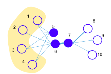
LINE is another interesting approach. The authors claim that LINE optimizes an objective that takes into account both the local and global structure of the graph when learning the embeddings of nodes. It does so by maximizing the embedding similarities between pairs of nodes with first-order proximity (i.e. preserving the local structure) and second-order proximity (i.e. preserving the global structure). The figure below demonstrates the 2 orders of proximity.
Training
In simple words, LINE defines a node (i.e. decides the embedding of a node) by making it similar to its first- and second-order proximity neighbors, while at the same time making it different from other, far-away nodes.
To make neighboring nodes similar, LINE repeatedly samples an edge (in cases of first-order proximity) or a path of length 2 (in cases of second-order proximity) in the graph and maximizes the dot product of the 2 end points’ embeddings. We remind the reader that we can think of the embeddings as normalized vectors, and thus, the larger the dot product the more similar the 2 embeddings (mind the Cosine similarity).
To make far-away nodes different, LINE, on the other hand, samples far-away pairs of nodes and minimizes their end points’ embeddings. This trick is a slight modification of Negative Sampling, as described earlier in this article.
As a side note, if the edges in the graph are weighted, we can do weighted samplings of edges and paths according to the edge weights. This preserves the importance of edges in the graph when encoding the nodes.
As an implementation detail, LINE optimizes for the first- and second-order proximity separately, then concatenates the results to get the final embeddings of the nodes.
Experimental results
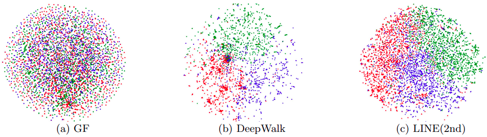
The authors evaluate LINE on 3 different tasks: word analogy, document classification in graphs, and compression for visualization. For the first 2 tasks, LINE outperforms then-SOTA models like Skip-gram [1], DeepWalk [14], and GF (Graph Factorization) [18]. For the last task, the result is compared with GF and DeepWalk and is shown in the figure below (read the figure caption for more details). Qualitatively, we can see that the compression given by t-SNE on the embeddings from LINE is much more meaningful and reasonable than the other 2 methods.
node2Vec
node2vec: Scalable Feature Learning for Networks, Grover and Leskovec
This is another paper that showed improvement in transforming from nodes to vectors. Its goal is to learn embeddings of nodes that preserve the similarity between (1) nodes in the same community as well as (2) nodes in different communities but have similar roles. The figure below illustrates these 2 types of similarities.
Training
Similar to DeepWalk [14], this work also leverages random walks and Skip-gram to learn embeddings of nodes. The random walks generate paths (or sequences of nodes) from the graph, which are treated similarly to sentences, while each node is analogous to a word. The Skip-gram model is then used to learn the embeddings of nodes, ensuring nodes that appear in similar neighborhoods have similar embeddings. The difference to (or improvement over) DeepWalk is the use of second-order biased random walks instead of just the original random walks.
This means when making the decision on what node to walk to next, the probability of selecting the next node depends on the distance from that next node to the previous node. For example, look at the figure below.
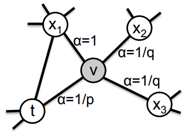
The figure illustrates the situation when the walk just traversed the edge  and is now staying at
  .
.  specifies the unnormalized probability of going to the next node, this probability for the neighbors of depends on the distance from them to the last node
  .
.

where:
 is the unnormalized probability to choose
  as the next node in the walk,
 is the distance between 2 nodes and ,
 and
and  are 2 hyper-parameters to control the behavior of the walks.
High-level speaking, this random walk strategy is somewhat a hybrid of DFS (as in DeepWalk) and BFS (similar to LINE [15]). How to assign values to these 2 hyper-parameters depends on the task and validation performance. (Note that by adjusting and , we can also replicate the DFS and BFS random walk strategies.)
Experimental results
The authors tested node2vec on 3 datasets for the task of node classification. In all experiments, node2vec showed superior performance against DeepWalk and LINE.
In this paper, the authors also suggest a simple way to obtain the representation of edges. For an edge  that connects 2 nodes (,
  ), they find that having
 vector(e) = Hadamard(vector(x), vector(y)) (Hadamard product is the element-wise product of 2 similar-size vectors) gives the best performance for all demonstrated edge-based prediction tasks.
Metapath2Vec
Metapath2vec: Scalable Representation Learning for Heterogeneous Networks, Dong and Chawla
Different from DeepWalk [14], LINE [15], and node2vec [16] which only focus on homogeneous graphs, metapath2vec is specifically designed to work on heterogeneous graphs whose nodes and edges may have multiple types.
Training
Similar to most other Node2Vec approaches, metapath2vec also makes use of random walks and Skip-gram for its embedding optimization process. However, the random walks here are not allowed to be truly random, but they need to follow a pre-defined structure of the node-/edge-type sequence.
To make things more concrete, let us take the academic publication graph as an example. In this graph, nodes can be of 1 of the 3 types (author, paper, venue, abbreviated by A, P, and V, respectively) while there are 2 types of edges (a publish edge connects A-P, P-V; and a coauthor edge connects A-A). An exemplar graph is shown in the figure below.
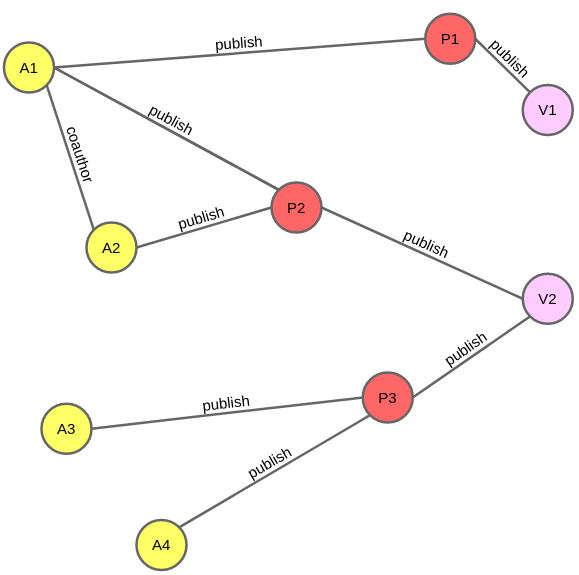
An essential hyper-parameter we need to decide for metapath2vec is the meta-path scheme, which describes the structure of the node-/edge types that the random walks should follow. For example, a meta-path scheme could be A - publish - P - publish - V - publish - P - publish - A. This scheme captures the publishing-in-the-same-venue relationship between authors. The walks generated by the algorithm need to follow this scheme, i.e. start at an author node, then follow a publish edge to a paper node, and so on, until it finishes at an author node. All these walks are then fed to Skip-gram to learn the embeddings of nodes, similar to in DeepWalk and node2vec.
The authors also suggest a modification of metapath2vec, called metapath2vec++ which alters the Skip-gram model a bit to further enable the simultaneous modeling of structural and semantic correlations of nodes in the graph. This change happens in the classification layer of Skip-gram, in which instead of applying Softmax on all classes as a whole, metapath2vec++ applies Softmax on each type of node separately.
Experimental results
Both variants of metapath2vec are tested on the 2 tasks of node classification and node clustering on heterogeneous graphs. They outperform prior type-ignorant methods (DeepWalk, LINE), showing that their utilization of types is indeed effective.
Edge2Vec
Edge2Vec techniques learn embeddings of edges in graphs.
Earlier in this article, we introduced a simple way to obtain the embedding of an edge by applying the Hadamard product to the embeddings of 2 nodes that this edge connects (the idea is from the node2vec paper [16]).
Another way is through a line graph of the original graph. Suppose we have a graph G, the line graph L(G) of G is constructed as: each node in L(G) corresponds to an edge in G, 2 nodes in L(G) are connected if and only if the corresponding 2 edges in G share one same node. Then, we compute the embeddings of nodes in L(G), which will give us the edge embeddings of G.
However, both methods above do not preserve all properties of edges and are not really performant (as compared to the method we are about to introduce next).
Edge2vec: Edge-based Social Network Embedding, Wang et al.
Since potentially the number of edges in a graph can be very large (can be as large as the square of the number of nodes in asymptotic terms), computing the embeddings for edges in an arbitrary graph can be very memory-consuming. To facilitate research, in this paper, the proposed method is trained and tested only on social network graphs, in which the average degree of nodes is small, resulting in reasonable numbers of edges.
The work defines 2 types of proximity: local and global proximities.
- Local Edge Proximity refers to whether 2 edges share one vertex.
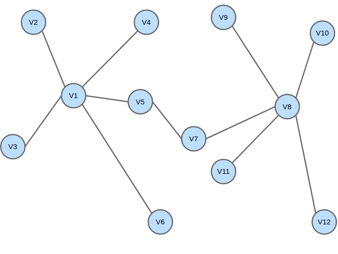
- Global Edge Proximity considers the distances between all pairs of edges. In simple terms, 2 edges are globally proximal if their distances to all nodes in the graphs are similar (see the figure below).
Training
The training process uses a deep autoencoder together with Skip-gram to preserve both types of proximity in edge embeddings.
For Local Edge Proximity, we first list out all pairs of adjacent edges (i.e. pairs of edges that share 1 vertex). The “co-occur” probability of 2 edges in all these pairs is then maximized by Skip-gram with Negative Sampling. As compared to text processing, this is analogous to maximizing the similarity of 2 words in the same context in word2vec [1].
For Global Edge Proximity, given an edge , we define a neighborhood vector  of length
  (where
  is the set of nodes) in which each value is in the range [0, 1], showing the information about how close each of the 2 ends of is to nodes in the graph. The closer the distance, the higher the corresponding value. The global proximity of 2 edges is the similarity of their neighborhood vectors (where the “similarity” can be quantified by, for example, Cosine similarity). Furthermore, to reduce the size of the neighborhood vectors, we compress them with a deep autoencoder.
Experimental results
The approach is evaluated on the tasks of link prediction, social tie sign prediction, and social tie direction prediction. In all experiments, it consistently outperforms other embedding-based deep models (DeepWalk [14], LINE [15], node2vec [16]).
Code2Vec
Computer programs can also be embedded.
While code embedding/understanding is an active research area with many recent works on it, in this article, we will introduce only 1 paper while leaving a comprehensive review of this field to a future thread.
code2vec: Learning Distributed Representations of Code, Alon et al.
The main objective of this method is to represent each code snippet by a fixed-length vector so that similar snippets result in similar vectors. Moreover, these vectors should also preserve the linear relationship (as in word2vec [1]). For example, given 3 functions equals, toLowerCase, and equalsIgnoreCase, we would like to have vector(equals) + vector(toLowerCase) = vector(equalsIgnoreCase).
Training
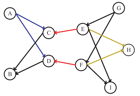
code2vec decomposes the code into paths in its Abstract syntax tree (AST) and then learns the representation of each path simultaneously with learning how to aggregate them using soft attention.
The AST of a code snippet is a tree that describes its computational structure. The figure below shows the AST of a simple piece of code.
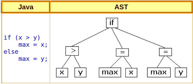
Within the scope of this paper, a path in the AST is a walk that connects 2 leaves of the tree without repeating any node (and thus there is only 1 path connecting any pair of nodes).
At first, we randomly initialize 2 matrices, one for the embeddings of paths and the other for the embeddings of nodes.
A path is characterized by the list of nodes and the directions of the edges that connect these nodes (directions can be either up or down the AST). As an implementation detail, only the most frequent paths in the training data are considered, the vocabulary size of paths is 1M. A node is characterized by its type and name.
A path-context representation is a concatenation of 3 vectors: that path’s vector and the 2 leaves’ vectors. Finally, a code snippet is represented by a random subset of path-context extracted from the AST.
There is a global context vector a for attention. Note that the attention here is global and is not similar to the self-attention mechanism from, e.g. the Transformer [21].
The path embeddings, node embeddings, and the global context vector a are jointly trained with gradient descent for the objective of classifying function names given function codes. In this process, the steps are summarized below:
- Given a function code, we build an AST.
- From the AST, a subset of
context-paths are then randomly extracted. - Each
context-pathis then vectorized as specified earlier. - This subset of
context-pathvectors are fed through a neural network (with an integrated attention mechanism) to predict their corresponding function name. - After the network converges, we get the learned embeddings for all nodes and paths, as well as
context-paths. These are used in the future when we want to embed new functions.
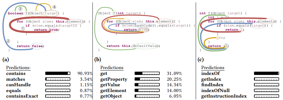
Experimental results
Being tested on the task of function name prediction, code2vec sharply outperforms existing approaches which use Path + Conditional Random Fields, or LSTM/CNN + attention.
Data2Vec
data2vec: A General Framework for Self-supervised Learning in Speech, Vision and Language, Baevski et al.
Last but not least, we introduce a recent work from Meta. Interestingly, this proposed approach can transform multiple modalities (texts, images, and voice) into vectors using the same training scheme while still maintaining SOTA performance.
Note, however, that each modality needs to be processed alone (i.e. not at the same time). The model can not yet take in multiple modalities at once.
Training
As a one-sentence summary, the approach uses the off-the-shelf transformer architecture with the pretraining objective to predict the representation of the original input given the masked input.
There are 2 models: teacher and student, both have the same architecture (the transformer) and size, but different weights. The input to the teacher is always the original data, while input for the student is masked data. At each time step, the student learns to mimic the average of the last K layers of the teacher, while the teacher parameters are updated as the exponential moving average of the student. High-level speaking, we try to make the encoding of the original input and of the masked input as similar as possible.
Notice that these learned embeddings are contextualized in a different way from well-known models like BERT [6]. In BERT, the target for each masked token is a fixed (correct) token, while in data2vec, the target for each sequence is a vector representation that changes depending on the context.
Also, while the training scheme is the same regardless of input modality, we still have different preprocessing for each type of input data. For images, we use the ViT-strategy [13] of encoding an image as a sequence of patches, each spanning 16×16 pixels. For voice, we use a multi-layer 1-D convolutional neural network that maps 16 kHz waveforms to 50 Hz representation (to reduce the input sequence length). For texts, we split the input into sub-words and encode them with embedding vectors.
The input is then masked for 15%, 60%, and 49% for texts, images, and voice, respectively, before being given to the student network.
The figure below illustrates the workflow of data2vec.

Experimental results
data2vec archives SOTA performance on all 3 modalities. For image classification and speech recognition, it noticeably beats prior SOTA approaches. For text data, its results on the GLUE tasks are comparable to that of BERT [6] and RoBERTa [23].
References:
- [1] Efficient Estimation of Word Representations in Vector Space, Mikolov et al. (2013), paper.
- [2] Distributed Representations of Words and Phrases and their Compositionality, Mikolov et al. (2013), paper.
- [3] Hierarchical Probabilistic Neural Network Language Model, Morin and Bengio (2005), paper.
- [4] Glove: Global vectors for word representation, Pennington et al (2014), paper.
- [5] Enriching Word Vectors with Subword Information, Bojanowski et al. (2017), paper.
- [6] BERT: Pre-training of Deep Bidirectional Transformers for Language Understanding, Devlin et al. (2018), paper.
- [7] Distributed Representations of Sentences and Document, Le and Mikolov (2014), paper.
- [8] Sentence-BERT: Sentence Embeddings using Siamese BERT-Networks, Reimers and Gurevych (2019), paper.
- [9] ImageNet Classification with Deep Convolutional Neural Networks, Krizhevsky et al. (2012), paper.
- [10] Very Deep Convolutional Networks for Large-Scale Image Recognition, Simonyan and Zisserman (2014), paper.
- [11] Deep Residual Learning for Image Recognition, He and Zhang (2016), paper.
- [12] EfficientNet: Rethinking Model Scaling for Convolutional Neural Networks, Tan and Le (2019), paper.
- [13] An Image is Worth 16×16 Words: Transformers for Image Recognition at Scale, Dosovitskiy et al. (2020), paper.
- [14] DeepWalk: Online Learning of Social Representations, Perozzi et al. (2014), paper.
- [15] LINE: Large-scale Information Network Embedding, Tang et al. (2015), paper.
- [16] node2vec: Scalable Feature Learning for Networks, Grover and Leskovec (2016), paper.
- [17] Metapath2vec: Scalable Representation Learning for Heterogeneous Networks, Dong and Chawla (2017), paper.
- [18] Distributed large-scale natural graph factorization, Ahmed et al. (2013), paper.
- [19] Edge2vec: Edge-based Social Network Embedding, Wang et al. (2020), paper.
- [20] code2vec: Learning Distributed Representations of Code, Alon et al. (2019), paper.
- [21] Attention is all you need, Vaswani et al. (2017), paper.
- [22] data2vec: A General Framework for Self-supervised Learning in Speech, Vision and Language, Baevski et al. (2022), paper.
- [23] Roberta: A robustly optimized BERT pretraining approach, Liu et al. (2019), paper.
- [24] SentEval: An Evaluation Toolkit for Universal Sentence Representations, Conneau and Kiela (2018), paper.
- [25] Supervised Learning of Universal Sentence Representations from Natural Language Inference Data, Conneau et al. (2017), paper.
- [26] Universal Sentence Encoder, Cer et al. (2018), paper.