SQL - aggregate functions

Aggregate functions are very useful and popular in database queries. These functions may be general-purpose: SUM, AVG, COUNT, MAX, MIN; concatenative: ARRAY_AGG, STRING_AGG; be for statistics: CORR, STDDEV_SAMP, STDDEV_POP, VAR_SAMP, VAR_POP; be for ordered-sets: MODE, PERCENTILE_CONT; for ranking: RANK, DENSE_RANK, PERCENT_RANK, CUME_DIST; etc. There are many other aggregate functions, however, these ones seem to be the most widely-used and worth our attention at the beginning steps into Database.

There are also 2 clauses being very important for aggregation, which are GROUP BY and HAVING – to be elaborated shortly.

Table of content
General-purpose Aggregation
$\mapsto$ SUM and AVG
$\mapsto$ COUNT
$\mapsto$ MAX and MIN
Concatenative Aggregation
$\mapsto$ ARRAY_AGG
$\mapsto$ STRING_AGG
Aggregation for Statistics
$\mapsto$ CORR
$\mapsto$ STDDEV_SAMP, STDDEV_POP, VAR_SAMP, VAR_POP
Ordered-set Aggregation
$\mapsto$ MODE
$\mapsto$ PERCENTILE_CONT
Hypothetical-set Aggregation
$\mapsto$ RANK
$\mapsto$ DENSE_RANK
$\mapsto$ PERCENT_RANK
$\mapsto$ CUME_DIST

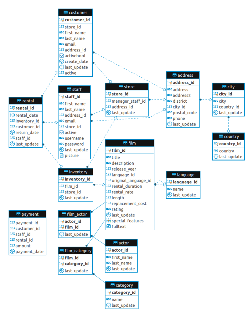
For illustrative purposes, we will be using the Pagila database, which is a port of the Sakila database (for MySQL) to Postgresql – the SQL version of this blog post. Pagila can be downloaded from here.

General-purpose Aggregation

SUM and AVG

Suppose we own a guesthouse, our service has been running for a month and generates some profits. Today, we open our computer, access our database and query the total income received. In this case, we use the SUM aggregate function. On the other hand, if we want to see how much, on average, a customer pays us for their booking, we should use the AVG function.

Example 1:

In this example, let’s calculate the total replacement cost for all films.

SELECT SUM(replacement_cost)
FROM film;

sum
19984.00

Note that for aggregate functions, all NULL values are excluded from the computation.

Example 2:

Let’s compute the average replacement cost, however, to make it harder, we compute the average replacement cost for each unique value of the length variable.

Now is when we should make use of the GROUP BY clause. Normally (i.e. without GROUP BY), the AVG function will calculate the average for all replacement costs in the table. Yet, with GROUP BY col_name, all rows with the same value for col_name are put into 1 group, then the average for each group is computed.

GROUP BY is placed after WHERE clause (if any) and before ORDER BY clause.

SELECT length, AVG(replacement_cost) AS "Average replacement_cost by length"
FROM film 
GROUP BY length
ORDER BY length;

length	Average replacement_cost by length
46	23.7900000000000000
47	20.1328571428571429
48	17.8990909090909091
49	18.5900000000000000
50	18.5455555555555556
51	21.1328571428571429
52	19.1328571428571429
53	21.5455555555555556
54	15.8233333333333333
55	17.4900000000000000

(There is a total of 140 rows, corresponding to 140 different values of length.)

Example 3:

However, we only want to see the replacement costs for films whose lengths are at least 90 minutes, thus we add a HAVING clause after the GROUP BY.

SELECT length, AVG(replacement_cost) AS "Average replacement_cost by length"
FROM film 
GROUP BY length
HAVING length >= 90
ORDER BY length;

length	Average replacement_cost by length
90	17.7900000000000000
91	18.1566666666666667
92	17.3536363636363636
93	20.6150000000000000
94	21.7400000000000000
95	18.9900000000000000
96	19.9900000000000000
97	15.7400000000000000
98	20.7400000000000000
99	20.7400000000000000

(There is a total of 96 rows.)

Note that HAVING acts very similar to the WHERE clause in terms that they both take in a boolean condition and filter the data, assuring that only the rows satisfying the condition are kept while the others are discarded. The only difference is HAVING is used in accompany with GROUP BY, i.e. WHERE is executed before grouping, while HAVING is executed after.

COUNT

The COUNT(expression) function, as per its name, returns the count of non-null values of the expression inputted.

Example 1:

SELECT COUNT(film_id) 
FROM film;

count
1000

Example 2:

Let’s query the counts of address and address2 in the table address. We will see that the 2 counts are different, since there are some NULL values in address2 and COUNT doesn’t include NULL values.

SELECT COUNT(address) AS count_1
     , COUNT(address2) AS count_2
FROM address;

count_1	count_2
603	599

Example 3:

When we just want to count the number of rows, the popular choices are COUNT(1) and COUNT(*), they both provide the same result with equal performance (equal processing time).

SELECT COUNT(1) 
FROM film;

count
1000

Example 4:

Note that COUNT does count the duplicated values. To count only the unique values, we use COUNT(DISTINCT expression).

Let’s count the number of rating categories:

SELECT COUNT(DISTINCT rating) 
FROM film;

count
5

MAX and MIN

Example 1:

Get the register date of the first customer (using create_date).

SELECT MIN(create_date)
FROM customer;

min
2017-02-14

Example 2:

Over the customers who ever spent more than 10$ for a single payment, find their lastest payment date.

SELECT customer_id, MAX(payment_date)
FROM payment
WHERE amount > 10
GROUP BY customer_id;

customer_id	max
116	2017-03-21 22:02:26
87	2017-03-20 19:42:24
477	2017-04-28 09:54:05
481	2017-04-08 08:40:11
550	2017-03-19 09:55:58
272	2017-04-30 08:54:45
304	2017-01-25 20:27:24
448	2017-04-30 10:27:16
511	2017-02-20 06:07:59
426	2017-04-30 21:58:17

(There is a total of 107 rows.)

Concatenative Aggregation

ARRAY_AGG

This function collects all the values and outputs an array of those values.

Example 1:

For each customer, get the list of all inventories he/she has made a rent. Show a sample of 10 first customers.

SELECT customer_id, ARRAY_AGG(inventory_id)
FROM rental
GROUP BY customer_id
LIMIT 10;

customer_id	array_agg
1	{14,3019,312,197,2785,2465,3021,1092,3497,3232,108,4566,1330,2639,3726,4020,1449,2269,2219,726,4249,797,1443,4497,921,1446,1021,1440,1558,1407,4268,3486}
2	{805,2053,2179,1090,1521,4038,2760,1382,4116,488,1937,654,3418,1149,4030,2377,4570,4088,138,626,3164,352,741,3142,2898,2060,3084}
3	{3241,4315,579,3261,3292,4560,3913,3328,1704,1984,2829,116,2526,1675,1182,2058,3917,2575,1685,1427,910,390,2468,3464,346,2150}
4	{4311,1075,165,280,3071,2553,57,185,97,4117,2495,3587,4385,3373,1976,3308,2980,2065,2479,984,132,3822}
5	{3482,1522,3022,61,169,1595,1574,1434,4364,2153,416,28,3998,3387,2623,711,2466,3333,1871,1183,1299,600,4323,1105,957,4400,2348,4124,1192,2177,4376,4463,3701,111,301,2587,3277,92}
6	{1818,2565,2085,98,1291,3617,3693,1929,1686,3136,2363,3938,731,1670,2858,3837,1261,3804,375,1325,3544,2686,2699,3317,3692,3952,1290,3888}
7	{3424,3929,75,2155,714,468,4374,3109,3318,1822,3645,3920,2877,3913,3024,1580,3104,2484,2272,2368,2812,2803,739,1512,4042,4045,1393,2866,4278,1950,2441,3480,3123}
8	{1907,187,971,1503,3153,8,1979,4054,2520,2522,2195,2270,2189,4511,3877,2388,2937,1936,2773,1841,2867,172,3278,4275}
9	{3483,2052,2435,2312,1395,981,3150,2484,373,2772,2279,4279,3926,886,3540,2756,4265,3790,2118,762,3773,4127,397}
10	{3891,2247,50,3826,2869,3834,67,4450,4326,1783,2968,1711,2937,418,1569,3086,4430,1767,749,2793,1866,3731,2570,80,1015}

Example 2:

The outputted arrays in Example 1 have their values unsorted, make them sorted.

SELECT customer_id, ARRAY_AGG(inventory_id ORDER BY inventory_id)
FROM rental
GROUP BY customer_id
LIMIT 10;

customer_id	array_agg
1	{14,108,197,312,726,797,921,1021,1092,1330,1407,1440,1443,1446,1449,1558,2219,2269,2465,2639,2785,3019,3021,3232,3486,3497,3726,4020,4249,4268,4497,4566}
2	{138,352,488,626,654,741,805,1090,1149,1382,1521,1937,2053,2060,2179,2377,2760,2898,3084,3142,3164,3418,4030,4038,4088,4116,4570}
3	{116,346,390,579,910,1182,1427,1675,1685,1704,1984,2058,2150,2468,2526,2575,2829,3241,3261,3292,3328,3464,3913,3917,4315,4560}
4	{57,97,132,165,185,280,984,1075,1976,2065,2479,2495,2553,2980,3071,3308,3373,3587,3822,4117,4311,4385}
5	{28,61,92,111,169,301,416,600,711,957,1105,1183,1192,1299,1434,1522,1574,1595,1871,2153,2177,2348,2466,2587,2623,3022,3277,3333,3387,3482,3701,3998,4124,4323,4364,4376,4400,4463}
6	{98,375,731,1261,1290,1291,1325,1670,1686,1818,1929,2085,2363,2565,2686,2699,2858,3136,3317,3544,3617,3692,3693,3804,3837,3888,3938,3952}
7	{75,468,714,739,1393,1512,1580,1822,1950,2155,2272,2368,2441,2484,2803,2812,2866,2877,3024,3104,3109,3123,3318,3424,3480,3645,3913,3920,3929,4042,4045,4278,4374}
8	{8,172,187,971,1503,1841,1907,1936,1979,2189,2195,2270,2388,2520,2522,2773,2867,2937,3153,3278,3877,4054,4275,4511}
9	{373,397,762,886,981,1395,2052,2118,2279,2312,2435,2484,2756,2772,3150,3483,3540,3773,3790,3926,4127,4265,4279}
10	{50,67,80,418,749,1015,1569,1711,1767,1783,1866,2247,2570,2793,2869,2937,2968,3086,3731,3826,3834,3891,4326,4430,4450}

Example 3:

For each customer, list all staff who served him/her. Show a sample of the first 10 customers. Remember to show each staff_id at most once for each customer.

SELECT customer_id, ARRAY_AGG(DISTINCT staff_id)
FROM rental
GROUP BY customer_id
LIMIT 10;

customer_id	array_agg
1	{1,2}
2	{1,2}
3	{1,2}
4	{1,2}
5	{1,2}
6	{1,2}
7	{1,2}
8	{1,2}
9	{1,2}
10	{1,2}

STRING_AGG

The STRING_AGG(expression, delimiter) also collects a list of values, however it then concatenate them together into a string and return this big string.

Example 1:

For each country_id, get all of its cities in the database, the cities should be listed in alphabetical order. Show a sample of the first 10 cities.

SELECT country_id, STRING_AGG(city, ', ' ORDER BY city)
FROM city
GROUP BY country_id
LIMIT 10;

country_id	string_agg
1	Kabul
2	Batna, Bchar, Skikda
3	Tafuna
4	Benguela, Namibe
5	South Hill
6	Almirante Brown, Avellaneda, Baha Blanca, Crdoba, Escobar, Ezeiza, La Plata, Merlo, Quilmes, San Miguel de Tucumn, Santa F, Tandil, Vicente Lpez
7	Yerevan
8	Woodridge
9	Graz, Linz, Salzburg
10	Baku, Sumqayit

Aggregation for Statistics

CORR

The CORR(expression_1, expression_2) function outputs the Pearson correlation coefficient of the 2 expressions over the current data (or group).

Example 1:

Calculate the correlation between film length and rental_duration to see if customers need more time to watch a longer film.

SELECT CORR(rental_duration, length)
FROM film;

corr
0.061586079089206866

We do have a positive correlation here, nevertheless, the value is quite small.

VAR_SAMP

The VAR_SAMP(expression) returns the sample variance of the input values, we can use this to measure the variability of a column.

Example 1:

Get the sample variance of rental duration for each distinct film length. Show a sample of the 10 shortest lengths.

SELECT length, VAR_SAMP(rental_duration) AS "var of rental_duration"
FROM film
GROUP BY length
ORDER BY length
LIMIT 10;

length	var of rental_duration
46	2.2000000000000000
47	2.2380952380952381
48	3.0181818181818182
49	2.2000000000000000
50	1.9444444444444444
51	1.9047619047619048
52	2.3333333333333333
53	2.0000000000000000
54	1.5000000000000000
55	4.5000000000000000

Example 2:

Apart from VAR_SAMP, we also have VAR_POP (the population variance of input data), STDDEV_SAMP (the sample standard deviation of input data, which equals the square-root of VAR_SAMP), STDDEV_POP (the square-root of VAR_POP).

In this example, we compute the sample standard deviation of the payment amount for each customer. Show a sample of the customers with id from 50 to 60, in increasing order of id.

SELECT customer_id, STDDEV_SAMP(amount) AS "std of amount"
FROM payment
GROUP BY customer_id
HAVING customer_id >= 50
   AND customer_id <= 60
ORDER BY customer_id;

customer_id	std of amount
50	2.5911351266716643
51	2.3264780248263683
52	2.1009029257555609
53	2.3238400909618506
54	2.1289352729120826
55	2.1275401432900819
56	2.4095562716123954
57	2.9212610690874983
58	2.6557438367734626
59	1.6131881356080347
60	2.5295010397712988

Ordered-set Aggregation

MODE

MODE() WITHIN GROUP (ORDER BY sort_expression) returns the most frequent value amongst input values (NULL will not be selected).

Example 1:

Find the most popular length of films.

SELECT MODE() WITHIN GROUP (ORDER BY length)
FROM film;

mode
85

PERCENTILE_CONT

The function PERCENTILE_CONT(fraction) WITHIN GROUP(ORDER BY sort_expression) returns the value at the given fraction percentile of the inputs. If needed, an interpolation between adjacent values will be made.

The most frequent fractions used for this function are 0.25 (the Q1), 0.5 (the median, Q2) and 0.75 (the Q3).

Example 1:

Get the median amount of payment for each customer. Show 10 customers with the highest median pay.

SELECT customer_id
     , PERCENTILE_CONT(0.5) WITHIN GROUP (ORDER BY amount) AS "median pay"
FROM payment
GROUP BY customer_id
ORDER BY "median pay" DESC
LIMIT 10;

customer_id	median pay
321	5.99
187	5.49
19	4.99
14	4.99
3	4.99
7	4.99
9	4.99
2	4.99
13	4.99
11	4.99

Hypothetical-set Aggregation

RANK

The function RANK(args) WITHIN GROUP (ORDER BY sorted_args) add a row containing the args to the table, rank the table by sorted_args and then output the rank of that newly added row.

Note that the rank generates gaps for duplicated rows. For example, rank [5, 9, 9, 13, 15, 15, 15, 100] gives [1, 2, 2, 4, 5, 5, 5, 8].

Example 1:

When we add a film with a length of 120 minutes to the table, then what is its rank in terms of length?

SELECT RANK(120) WITHIN GROUP (ORDER BY length)
FROM film;

rank
535

DENSE_RANK

This function is very similar to RANK, the difference is that it uses dense-rank – the dense rank function does not generate gaps for duplicated rows. For example, dense-rank [5, 9, 9, 13, 15, 15, 15, 100] gives [1, 2, 2, 3, 4, 4, 4, 5].

Example 1:

When we add a film with a length of 120 minutes to the table, then what is its dense-rank in terms of length?

SELECT DENSE_RANK(120) WITHIN GROUP (ORDER BY length)
FROM film;

dense_rank
75

PERCENT_RANK

This function is also similar to RANK, it does exactly what RANK does, then normalizes the output value. PERCENT_RANK normalizes the output to the range [0, 1].

Example 1:

SELECT PERCENT_RANK(120) WITHIN GROUP (ORDER BY length)
FROM film;

percent_rank
0.534

CUME_DIST

The CUME_DIST calculates the cumulative distribution. It is computed by dividing the number of rows smaller than or equal to it (including itself) for the total number of rows. Thus its output is in the range [1/n, n].

Example 1:

SELECT CUME_DIST(120) WITHIN GROUP (ORDER BY length)
FROM film;

cume_dist
0.5434565434565435

Summary

In this blog post, we introduced the common aggregate functions being used in Postgresql. Those are:

General Purpose Aggregations
SUM(expression), AVG(expression)	Return the sum or average of input values.
COUNT(expression)	Return the count number of input values.
MAX(expression), MIN(expression)	Return the maximum or minimum of input values.
Concatenative Aggregations
ARRAY_AGG(expression)	Return an array consisting of input values.
STRING_AGG(expression, delimiter)	Return a string which is the join of input values by the delimiter.
Aggregations for Statistics
CORR(expression_1, expression_2)	Return the correlation of the 2 lists of values.
STDDEV_SAMP, STDDEV_POP, VAR_SAMP, VAR_POP (expression)	Return the sample (or population) standard deviation (or variance) of input values.
Ordered-set Aggregations
MODE() WITHIN GROUP (ORDER BY sort_expression)	Return the most frequent value amongst input values.
PERCENTILE_CONT(fraction) WITHIN GROUP(ORDER BY sort_expression)	Return the value corresponding to the inputted fraction percentile.
Hypothetical-set Aggregation
RANK(args) WITHIN GROUP (ORDER BY sorted_args)	Return the rank of the args if it is inserted into the data.
DENSE_RANK(args) WITHIN GROUP (ORDER BY sorted_args)	Return the dense-rank of the args if it is inserted into the data.
PERCENT_RANK (args) WITHIN GROUP (ORDER BY sorted_args)	Return the normalized rank of the args if it is inserted into the data.
CUME_DIST (args) WITHIN GROUP (ORDER BY sorted_args)	Return the cumulative distribution up to that row.

References:

List of all aggregate functions in Postgresql: link
Paquier’s explanation of WITHIN GROUP: link

Tung M Phung's Blog

SQL – aggregate functions

General-purpose Aggregation

SUM and AVG

COUNT

MAX and MIN

Concatenative Aggregation

ARRAY_AGG

STRING_AGG

Aggregation for Statistics

CORR

VAR_SAMP

Ordered-set Aggregation

MODE

PERCENTILE_CONT

Hypothetical-set Aggregation

RANK

DENSE_RANK

PERCENT_RANK

CUME_DIST

Summary

Leave a ReplyCancel reply