
The new Coronavirus is spreading fiercely. At the time of this writing, more than 200 countries around the world have been invaded by this tiny species.
To monitor the status of nations on coping with this disease, the John Hopkins University attempted to collect data from various trustworthy sources (WHO, CDC, etc.) to analyze and publish this wonderful geo-map to show to the public.
A geo-map is, without a doubt, the most suitable visualization for the problem at hand. Apparently, this was a useful tool from before this virus exists, and probably be so even after the crisis comes to an end.
With that in mind, the goal of this post is to help you make familiar with this handy geo-map plot.
Here is our final result:
Let’s get started!
Data
First, we need to get the data.
Thanks to Johns Hopkins University, they have published and constantly updated their dataset on this Github repo. From there, we can download a csv data file for each day from Jan 22, 2020, onward.
For the purpose of this article, I use the statistics of March 30, 2020. However, as of the time you read this, there should probably be more updated records. Please feel free to take the lastest data for your practice.
Copy the data from the above source and save it to ./covid-20200330.csv.
Plotly
The Plotly library for Python has become increasingly popular these years. Its support for making interactive charts is exceptional.
Today, we will use its scattergeo plot, which, literally, is a scatter plot on a geo-map.
Action
First, we import the needed libraries. Pandas for loading the dataset and Plotly to visualize it.
import pandas as pd
import plotly.graph_objects as go
Note that from Plotly, we take the graph_objects, which is a low-level interface acting as a container (or builder) of plots.
Load the data to a Pandas data frame and take a look at the first rows:
data = pd.read_csv('./covid-20200330.csv')
print(data.head())
      FIPS     Admin2  Province_State Country_Region          Last_Update  \
0  45001.0  Abbeville  South Carolina             US  2020-03-30 22:52:45
1  22001.0     Acadia       Louisiana             US  2020-03-30 22:52:45
2  51001.0   Accomack        Virginia             US  2020-03-30 22:52:45
3  16001.0        Ada           Idaho             US  2020-03-30 22:52:45
4  19001.0      Adair            Iowa             US  2020-03-30 22:52:45

         Lat       Long_  Confirmed  Deaths  Recovered  Active  \
0  34.223334  -82.461707          3       0          0       0
1  30.295065  -92.414197         11       1          0       0
2  37.767072  -75.632346          6       0          0       0
3  43.452658 -116.241552        113       2          0       0
4  41.330756  -94.471059          1       0          0       0

                    Combined_Key
0  Abbeville, South Carolina, US
1          Acadia, Louisiana, US
2         Accomack, Virginia, US
3                 Ada, Idaho, US
4                Adair, Iowa, US
Among these 12 columns, what we need are:
Note that I do not use the Active column since it seems unreliable (at least for the US, in which it always gives 0). Instead, the number of active cases, if desired, can be calculated by subtracting the Deaths and Recovered from the Confirmed value.
If you screen through the data, you will see that some countries have their records on each state or city separately, while for the others, only 1 record is generated for the whole country, which seems not fair for comparison at all. To address this issue, we will group all rows belonging to the same country into one:
# sort by the number of confirmed cases
# in decreasing order.
data = data.sort_values(['Confirmed'], ascending=False)

# group records by country.
data = data.groupby('Country_Region').agg({'Lat': 'first',
                                           'Long_': 'first',
                                           'Confirmed': 'sum',
                                           'Deaths': 'sum',
                                           'Recovered': 'sum',
                                          })
data = data.reset_index()
Fair enough.
Now, let’s take a look at the markers (the circles representing the number of cases for each country), we have to take care of their sizes. The marker’s size of a country should be in proportion with its corresponding cases, obviously. A country with more patients than the other should also have a bigger circle.
However, as some countries have hundreds of thousands of cases while some others contain only several, if the circle size is linearly correlated with this value, the low-number countries will have their marker too small, even invisible for us to see. Thus, we should scale the marker size by a nonlinear scale of the number of cases. Below, I use the square-root:
# define a scaling function
# this function helps adjust the size of markers on the plot.
scale_factor = max(data['Confirmed'])
def scaling(column, factor):
    return (column / factor) ** 0.5 * 50

# make representations of the number of cases
# using the above-defined scaling function.
data['Confirmed-ref'] = scaling(data['Confirmed'], scale_factor)
data['Ended-ref'] = scaling(data['Deaths'] + data['Recovered'], scale_factor)
data['Death-ref'] = scaling(data['Deaths'], scale_factor)
That is almost done with the pre-processing of data. There is only 1 more thing: we add a column that contains the information to be shown when hovering over the plot.
What information do you want to see from a marker? I would suggest the country name, the number of confirmed cases, recovered cases and deaths.
# make a summary for each country
# this will be shown as we hover over the markers on the plot.
data['summary'] = (
    '<b>'
    + 'Country: '
    + data['Country_Region']
    + '</b>'
    + '<br><br>'
    + 'Confirmed: '
    + data['Confirmed'].astype(str)
    + '<br>'
    + 'Recovered: '
    + data['Recovered'].astype(str)
    + '<br>'
    + 'Deaths: '
    + data['Deaths'].astype(str)
    )
Ok, it’s time for Plotly.
To begin with, we will make a plot of the confirmed cases. On a world map, for each country in our dataset, a circle (marker) is put on the corresponding co-ordinate (lat – long). The size and the color of the markers vary depending on the number of confirmed cases. Countries with lots of cases are represented by big red markers while the ones with fewer infections are small and yellow.
# make a figure
fig = go.Figure()

# plot the number of confirmed cases.
fig.add_trace(go.Scattergeo(
    lat = data['Lat'],
    lon = data['Long_'],
    marker = dict(
        size = data['Confirmed-ref'],
        color = data['Confirmed-ref'],
        colorscale = [[0, 'rgb(255,255,0)'],
                      [1, 'rgb(255,0,0)']
                     ],
        opacity = 1,
        ),
    text = data['summary'],
    hovertemplate = '%{text} <extra></extra>',
    ))

# draw the border of each country.
fig.update_geos(
    showcountries=True
)

# show figure
fig.show()
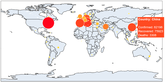
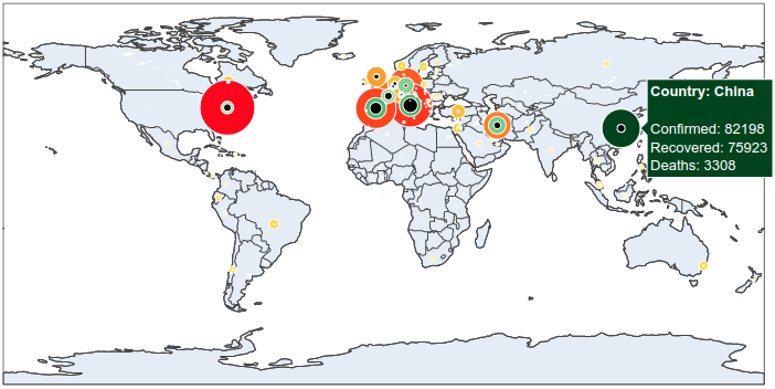
It is now simple to reproduce the map we have at the beginning of the article. We just have to add to this map the number of recovered and death cases.
# make a figure
fig = go.Figure()

# plot the number of confirmed cases.
fig.add_trace(go.Scattergeo(
    lat = data['Lat'],
    lon = data['Long_'],
    marker = dict(
        size = data['Confirmed-ref'],
        color = data['Confirmed-ref'],
        colorscale = [[0, 'rgb(255,255,0)'],
                      [1, 'rgb(255,0,0)']
                     ],
        opacity = 1,
        ),
    text = data['summary'],
    hovertemplate = '%{text} <extra></extra>',
    ))

# plot the number of ended cases.
fig.add_trace(go.Scattergeo(
    lat = data['Lat'],
    lon = data['Long_'],
    marker = dict(
        size = data['Ended-ref'],
        color = data['Ended-ref'],
        colorscale = 'Greens',
        opacity = 1,
        ),
    text = data['summary'],
    hovertemplate = '%{text} <extra></extra>',
    ))

# plot the number of recovered cases.
fig.add_trace(go.Scattergeo(
    lat = data['Lat'],
    lon = data['Long_'],
    marker = dict(
        size = data['Death-ref'],
        color = 'black',
        opacity = 1,
        ),
    text = data['summary'],
    hovertemplate = '%{text} <extra></extra>',
    ))

# draw the border of each country.
fig.update_geos(
    showcountries=True
)

# show figure
fig.show()
And here we are done.
The complete code can be found on this repository.
References: