Subgroup Discovery: Beyond coverage and mean-shift

1. Introduction

Subgroup Discovery (SD) is the process of identifying a part of the data that stands out on some target variables. To measure the goodness of a subgroup, it is widely agreed that a trade-off between generality and exceptionality needs to be made. Traditionally, generality is usually approximated by the absolute (or relative) size of the subgroup while exceptionality is quantified as a function regarding the average difference in the target variable between the subgroup and the whole population. The Weighted Relative Accuracy [1] and the Impact measure [7] are such well-known evaluations for discrete and continuous target variables, respectively. However, recent research, including the work by Song et al. [6] and Boley et al. [2] points out that those metrics usually over-emphasize the role of size while understating the coherence, or the intra-consistency between data points in the subgroup, resulting in sub-optimal discovery. To make up for such sub-optimality, they propose new evaluation functions that take into account group divergence (Song et al.) and dispersion (Boley et al.).

In section 2, we first give a more detailed summary of the above-mentioned approaches before discussing their effectiveness. Another new idea involving representativeness by Kalofolias et al. [4] is introduced in Section 3. Lastly, a brief conclusion is given in Section 4.

2. Subgroup Discovery with Proper Scoring Rules and Dispersion-correction

2.1 Subgroup Discovery with Proper Scoring Rules

In the field of machine learning, proper scoring rules such as Log-loss and Brier Score have been, for a long time, the top-selling metrics for quantifying the fitness of predicted and ground-truth probabilities. Observing them being such successful in a related field, Song et al. [6] asked an intriguing question: why can’t they be applied in subgroup discovery? To be more specific, the authors look at SD as a medium to make a better summary of the data, while a summary can be naturally defined as the probability distribution of the (discrete) target values. Given a data population P, its best subgroup $Q^*$ is the subgroup $Q \subset P$ that minimize the total difference between the data points and the summary, while the difference is measured by a proper scoring rule, that is:

$\begin{aligned}Q^* = \underset{Q}{\arg\min} \quad \sum_{y_i \in Q} \Psi (s^Q, y_i) + \sum_{y_j \not\in Q} \Psi (s^\pi,y_j) \quad\quad \quad (1)\end{aligned}$

where $\Psi$ is a proper scoring rule, $s^\pi$ is the summary (i.e. average probability distribution of the target variable) of the population, $s^Q$ is the summary of a subgroup Q, $y_i$ and $y_j$ are the i-th and the j-th data point, respectively. Since $\Psi$ is proper, $\Psi (s^Q, y_i)$ is minimized when $y_i$ approaches $s^Q$ , which motivates the consistency of data points within the subgroup.

Geared with this idea, the authors further optimize the computation to concern the two generalization problems when a subgroup language is derived from a (small) training data and applied to future data: the uncertainty about the subgroup’s class distribution and about whether its actual distribution is different from the population. In the end, they propose 4 quality measures as the product of the set of 2 proper scoring rules, Brier and Log-loss, and whether to adjust for only the first or both of the above uncertainties:

$\begin{aligned}\phi_d(g) = m * d(\pi, \hat{\rho}), \quad\quad\quad\quad \phi_{PSR}(g) = m * d(\pi, \hat{\hat{\rho}})\end{aligned}$

where $\phi_d$ and $\phi_{PSR}$ are the measures that concern the first and both uncertainties, respectively; $m$ is the size of the subgroup, $\hat{\rho}$ and $\hat{\hat{\rho}}$ are the adjusted probability distributions of the subgroup for corresponding measures, $d$ is the divergence function which is different for different scoring rules. Note that these adjusted probability distributions can be thought of as a smoothing factor that can discourage the resulting subgroup from being very small in size.

Since the main goal of this research is basically to separate the data into 2 halves in order to improve the global summary, it is directly implied by Eq. (1) that this objective is achieved, at least in the training set. For the performance on test data, their experiments on 20 UCI datasets [6] also show encouraging results, as the searches using proposed measures outperform their counterparts (including Weighted Relative Accuracy, Chi-Squared, and methods based on Information gain) in most cases. Furthermore, the authors also try their approach on a general SD task, that is, to recognize an actual subgroup in the data. According to their experiment on a synthesis dataset, the four novel measures top the traditional methods by a great margin.

It is worth it to note that one of the datasets is artificial, and some (including myself) might not be a fan of experimental results on author-created datasets. While the process of generating this dataset looks legit, it is not rare that sometimes, some authors tend to cherry-pick from a bag of legit settings to get the one that is most beneficial for their purposes. However, as of my understanding, evaluating a SD approach is much harder than a supervised one, since there is usually no ground truth to be compared with, and in those cases, creating a synthesis dataset, as done by Song et al., is indeed necessary. Moreover, from the theoretical point of view, the research is persuasive in the sense that the authors reuse the very popular practice (i.e. the Proper scoring rules such as Brier score and Log-loss) from a closely related field with only small modifications to apply to SD. My subjective opinion is that for an approach that is (empirically) proved as good for a task A, and then if it shows some initial competence in another similar task B, it is very likely that this approach is actually suitable for both tasks, rather than just performing well on task B by coincidence.

2.2 Subgroup Discovery with Dispersion-correction

In contrast to the above method that is applied to SD with discrete target variables to improve the overall summary, the work by Boley et al. [2] focuses on data with numerical objective values and aims for extracting an interesting subgroup with disregard for the rest of the dataset. The authors want to explicitly address the problem of traditional approaches that the consistency of data points inside the group is rarely taken into account. They show that while the generality and central tendency (e.g. mean and median) are necessary, the dispersion of the subgroup is an equally critical measure. Formally, the subgroup quality measure function $f$ should be of the form:

$\begin{aligned}f(Q) = g(|Q|, c(Q), d(Q))\end{aligned}$

where $Q$ is a subgroup; $c$ is a central tendency function which often involves mean or median; $d$ is a dispersion function; and $g$ is a function that is monotonically increasing with the subgroup size, monotonically decreasing with the dispersion index given by $d$ , and depends on none other values except the central tendency index given by $c$ . While the idea already makes intuitive sense on its own, it helps to point out that it solves a problem of traditional methods, that they usually result in a subgroup with almost as high or even higher error than it of the population [2]. The authors also suggest making the computation of $c$ and $d$ to be around the median (instead of the mean), which not only makes the model more robust against outliers but also facilitates the use of the tight optimistic estimator [3, 5] in linear time to better prune the search space in the branch-and-bound scheme. To be more specific, let us rewrite the valuation function $f$ as:

$\begin{aligned}f(Q) = g(\text{dcc}(Q), \text{med}(Q)) \quad\quad \text{with} \quad\quad dcc(Q) = \left(\frac{|Q|}{|P|} - \frac{\text{smd}(Q)}{\text{smd}(P)}\right)_+\end{aligned}$

where $smd$ is the sum of absolute deviations from the median, and $med$ is a function on the median. Then, given a subgroup Q, the tight optimistic estimator of any refinement of Q can be computed in time linear to the size of Q, making it efficient to prune any branches with this estimator smaller than the actual valuation of the best candidate so far. Note that other forms of $dcc$ are also allowed, as long as they are linear and positively dependent on $|Q|$ and negatively dependent on $smd$ .

Regarding experimental results, the test on 25 datasets shows that in general, the dispersion-corrected objective measure usually results in a smaller but more coherent subgroup than the non-dispersion-corrected counterpart. Furthermore, empirical results also suggest that on average, dispersion-correction increases the relative lower confidence bound of predicting the target values for test data by at least 10 percent, which is a big improvement.

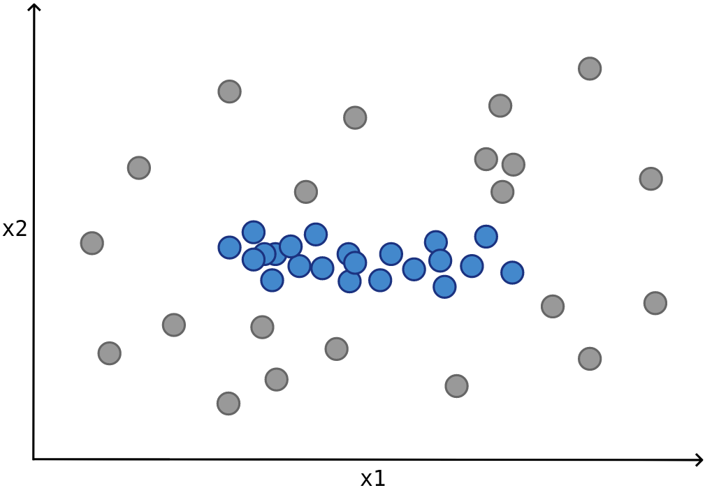
Overall, the major contribution of this research is that it not only proposes an intuitive yet effective theoretical approach to deal with the subgroup-coherence problem but also makes it practical with the efficiency of computing the tight optimistic estimator in linear time. In a sense, it dominates the traditional approaches (which only make use of the pure coverage and central tendency) in effectiveness, while being comparable in time complexity. One interesting trait to point out is that, depending on the purposes, it might be in favor to mine exceptional subgroups that have the same central tendency as the population (as illustrated in Fig. 1). While canonical objective functions fail to achieve for this case, the dispersion-corrected functions can still work well, e.g. by adjusting the $med$ factor to always return 1. The only minor downside of this correction is that to keep the time linear, it is required that computations are restricted to be around the median (and the sum of absolute deviations from the median), while the mean and variance are often more preferred, especially if the sensitivity to outliers is considered as a meaningful factor.

fig. 1 — Figure 1. Illustration of a subgroup with almost zero central tendency shift from the population. Given x2 as the target variable, the subgroup formed by the blue dots is not discoverable by functions that only consider the coverage and mean/median-shift. This interesting subgroup can, however, be recognized by dispersion-corrected measurements. Also, this (blue) subgroup is a poor representative of the population despite their similar mean/median.

2.3 Comparison of the two approaches

Even though both methods are designed to address the disproportionate issue of traditional approaches that consider only subgroup size and central tendency, they are actually very different in many aspects. Let us restate that while the work by Song et al. aims to SD with discrete targets, Boley et al. focus on numerical objective values. Moreover, the main goal of the former is to improve the global summary of the data, in contrast to the latter that only pays attention to the extracted subgroup without pertaining to the rest. To integrate group coherence into the evaluation functions, while Song et al. make modifications to the exceptionality factor (and keep the coverage factor untouched), the reverse is true to the other work, in which case the main correction is made on the coverage factor, while the exceptionality factor is only slightly modified (i.e. from mean-based to median-based). Another minor difference is that while the former reuses the widely-accepted metrics such as Log-loss and Brier Score, the latter takes a more adventurous choice to work with less-common measures like the median and $smd$ (compared to mean and variance). However, notice that the same dispersion-correction can also be applied to mean and variance if we are willing to pay the cost of quadratic time complexity for the tight optimistic estimator.

3. Representativeness

One more interesting idea we are going to review in this blog post is the work from Kalofolias et al. [4] which introduces representativeness, a measure of how a subgroup is distributionally similar to the population with regards to some variables. They argue that in many cases, we want to find out local factors that affect some (target) variables but in control for specific explanations. Those cases might vary from restraining the algorithm from outputting already-known knowledge to ensuring ethical fairness in classification. Being motivated by this idea, and since just simply removing the control variables is not very effective, they propose to adjust the evaluation function to include this representativeness factor. That is, if we call $f_{ct}$ our original (and arbitrary) function, its representativeness-corrected version is the function $f$ such that:

$\begin{aligned}f(Q) = f_{ct}(Q)^{1-\gamma} * f_r(Q)^\gamma \label{eq:2}\quad\quad\quad (2)\end{aligned}$

where $f_r(Q)$ is a function that quantifies the representativeness of (Q) with respect to the population P on some control variables, and $\gamma$ is the tuning parameter that regulates the trade-off between $f_r$ and $f_{ct}$ .

Since this idea is orthogonal to the approaches from Song et al. and Boley et al., it is perfectly reasonable to combine it with these two to make even stronger methods. Besides the above-mentioned benefits, another contribution from this representativeness-correction might be the ability to facilitate the discovery of overlapping meaningful subgroups. That is, to put in the context of mining multiple subgroups, the straightforward way to apply the above two approaches is to gradually extract one group at a time and exclude the found groups from the data that is used to mine subsequent groups. However, this process suffers from the problem that those mined subgroups are mutually exclusive (no data points belong to more than one group) and the formation of later groups is biased with regards to the absence of excluded data points. This problem is (at least partially) addressed by the integration of control variables, in which scenario we can replace the exclusion of found subgroups by introducing more control variables with regards to the subgroup languages that generated the former subgroups. From the technical point of view, the combination is also obviously possible, since we can just plug the objective function from Song et al. and Boley et al. to $f_{ct}$ in Eq. (2). Note, however, that the linear-time algorithm proposed by Boley et al. might get affected.

On the reverse side, given that the control variables could be either discrete or continuous, it is also rational that we try to apply the idea from the former two research to compute $f_r$ . To be more specific, in their design, Kalofolias et al. define $f_r$ as a function over the distance $d$ between the subgroup and the population, where $d(q, p) = \frac{1}{2} \sum_k |q_k - p_k|$ . This distance function might be directly changed to be based on proper scoring rules (as suggested by Song et al.) in the case of discrete values. Notice that the definition of representativeness of a subgroup Q is almost entirely equivalent (but negatively correlated) with its divergence from the population P. In the case the control variable is continuous, the distance $d$ should consider both the difference in the central value and dispersion since the shift in central tendency alone is far from enough to compare two distributions. Again, refer to Fig. 1 for an illustration.

4. Conclusion

In this work, we briefly summarize and analyze the ideas from three interesting papers in the field of subgroup discovery [2, 4, 6]. We describe how the goals of Song et al. and Boley et al. are similar even though their approaches are vastly different. We also give reasons to demonstrate that the representativeness factor by Kalofolias et al. can be a good companion to both of them and conversely, these two methods can also be adapted to improve the representativeness-correction.

References:

[1] Evaluation measures for multi-class subgroup discovery, Abudawood and Flach, 2009, pdf
[2] Identifying consistent statements about numerical data with dispersion-corrected subgroup discovery, Boley et al., 2017, pdf
[3] Tight optimistic estimates for fast subgroup discovery, Grosskreutz et al., 2008, pdf
[4] Efficiently discovering locally exceptional yet globally representative subgroups, Kalofolias et al., 2017, pdf
[5] Fast exhaustive subgroup discovery with numerical target concepts, Lemmerich et al., 2016, pdf
[6] Subgroup discovery with proper scoring rules, Song et al., 2016, pdf
[7] Discovering associations with numeric variables, Web, 2001, pdf

Tung M Phung's Blog