In this article, we are going to discuss some of the essential concepts from Information Theory. To facilitate learning, let us take the Titanic dataset for examples.
For simplication, we will only use 3 features:
Note that reading the code is optional. You can understand the whole content without the code.
import numpy as np
import pandas as pd

data = pd.read_csv('titanic_train.csv')
data = data[['Survived', 'Sex', 'Embarked']].dropna()
Information Content
The Information Content of a value measures how surprising that value is.
For example, suppose we have a biased coin which 90% of the time turns out to be head, while only 10% tail. If we toss that coin and it results in a head, is that event surprising? Not really. But if it shows a tail? Yes, because that event happens only 10% of the time, it is so unlikely to occur. Things that are surprising give us more information, thus they have higher Information Content. With this intuition, let’s look at the formal formula:

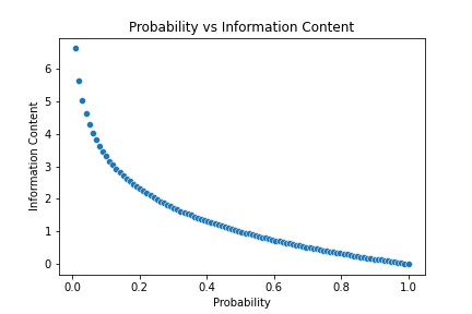
So the amount of information is defined to be the negative logarithm of its probability. While this formula does ensure that rarer values mean higher information content, it is not so intuitive how the logarithm is employed here. Why don’t we use a simpler formula, such as:

The answer is, the negative correlation between probability and information is just one of the qualifications, it is necessary but not enough. The value of  is also the expected number of bits to efficiently encode x.
Information Encoding
Encoding, or Compression, refers to the work that inputs some data and outputs a smaller-size sequence of bits that can represent that data.
Take the Embarked column for example. Here we have 889 instances, among those 644 are S, 168 are C, while the remaining 77 are Q. The question is: how can we map each of these 3 values to a bit sequence so that when we append all the 889 sequences, we get the shortest uniquely decodable compression?
For example, if we correspond S to 101, C to 0, Q to 11 , then the resulting compression will have  bits. Another encoding scheme is to map S to 0, Q to 11, and C to 10. In this case, the compression has a length of 1134, which is much better.
Furthermore, the latter encoding is actually equivalent to a Huffman tree, so it is the most efficient encoding we can have. In general, when we have more different values to be encoded, the best encoding algorithm will map a value to a bit-sequence whose length is approximately the negative of the logarithm of that value’s probability. For example, if any value x has a probability of occurrence p(x), then its encoded length is roughly .
As we have just demonstrated, the lower the probability of an event, the higher its information, and also the more bits we use to encode it. Thus, for convenience, we purposely quantify the amount of information by the number of encoding bits.
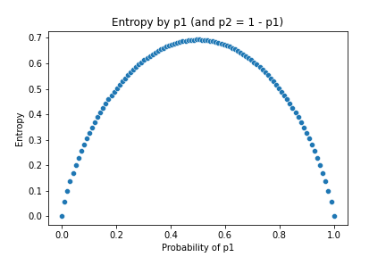
Entropy
The Entropy of a set is the average number of bits we need to encode each entry of that set.
For the Embarked column, as stated above, we encode S by 0, Q by 11, and C by 10. So what is its entropy? Some may compute the entropy as H = (1 + 2 + 2) / 3 = 5/3, but that is not true. Since the probability of each event is different, we cannot just take the mean of their bits. In this case, as S appears 644 times, C 168 times, and Q 77 times, their probability are  ,
,  , and
, and  , respectively. Thus, the entropy, or the average number of bits to encode one entry of this Embarked column is:

In general, since we can approximate the number of bits to encode x by , the formula for entropy is formally defined as:

In this case, if we plug the numbers in, we have  .
.
From another point of view, we can also call the Entropy as the Uncertainty of data. The intuition is that when the probability of entries are the same (i.e. they are uniformly distributed), the entropy is highest, meaning we know less about the data, or we are uncertain about the data. On the reserve side, when the distribution is skewed (i.e. some entries have significantly bigger probability while some have only small chance to occur), the entropy is low, meaning if we are given a random entry from the data, we are more certain what its value is.
from scipy.stats import entropy

def compute_entropy(sequence, base=2, axis=None):
    value, counts = np.unique(sequence, axis=axis, return_counts=True)
    return entropy(counts, base=base)

ent = compute_entropy(data['Embarked'].to_numpy())
print(f'Entropy of Embarked: {ent:.2}')
Entropy of Embarked: 1.1
Joint Entropy
The idea of Entropy can be generalized to more than 1 variable.
Let us compute the Entropy of both Embarked and Sex together. Since Embarked has 3 possible values (S, C, Q) while Sex has 2 possible values (male and female), there are in total 6 different combinations. The counts and relative probabilities of these combinations are given in Table 1.
| Value | Counts | Probability (approximation) |
| (‘C’, ‘female’) | 73 | 0.08 |
| (‘C’, ‘male’) | 95 | 0.11 |
| (‘Q’, ‘female’) | 36 | 0.04 |
| (‘Q’, ‘male’) | 41 | 0.05 |
| (‘S’, female’) | 203 | 0.23 |
| (‘S’, ‘male’) | 441 | 0.5 |
The Joint Entropy of Embarked and Sex is then:
![\begin{aligned} H(\text{Embarked, Sex}) &= \sum_{x \in \text{Embarked},y \in \text{Sex}} -p(x, y)\log p(x, y) \\&\approx - [0.08 \times log(0.08) + 0.11 \times log(0.11) \\ &+ 0.04 \times log(0.04) + 0.05 \times log(0.05) \\&+ 0.23 \times log(0.23) + 0.5 \times log(0.5)] \\&\approx 2.02\end{aligned}](https://tungmphung.com/wp-content/ql-cache/quicklatex.com-4a9fa6cd6e927fad881ce0ce6d1e83f7_l3.png "Rendered by QuickLaTeX.com")
That is the Joint Entropy (nothing more than the Entropy of a combination). One remark is that, say we have 2 variables A and B, then their joint entropy is always at least as large as any of A or B’s individual entropy. That is:

This makes sense since we should be at least as uncertain about 2 variables as we are uncertain about each of them. Furthermore, the equality occurs only when one of A and B has zero entropy (i.e. one of its values has probability 1 while all others have 0).
def compute_joint_entropy(p, q, verbose=False):
    joint_sequence = [(x, y) for x, y in zip(p, q)]

    if verbose:
        values, counts = np.unique(joint_sequence, axis=0, return_counts=True)
        probabilities = counts / sum(counts)
        print('values:', values)
        print('counts:', counts)
        print('probabilities:', probabilities)

    joint_ent = compute_entropy(joint_sequence, axis=0)
    return joint_ent

joint_ent = compute_joint_entropy(data['Embarked'], data['Sex'], verbose=False)
print(f'Joint Entropy of Embarked and Sex: {joint_ent:.2}')
Joint Entropy of Embarked and Sex: 2.0
Cross-Entropy
Above, we learned that the Entropy of a set is the average number of bits we need to encode an arbitrary value using its best encoding scheme. Now, we consider encoding one set A by the best encoding scheme of another set B. That is, we take a set B, calculate the probabilities of its entries to come up with the most efficient encoding algorithm, which can encode B to the shortest bit sequence. Then, we apply that algorithm to set A, what is the average number of bits do we need for each entry of A?
The answer is the Cross-Entropy of B relative to A, denoted by:

where A(x) is the probability of entry x in A and B(x) is the probability of entry x in B. Note that we assume A and B have the same set of values.
A more common way that people use to write the cross-entropy of B relative to A is: H(A, B). However, this is confusing since the same notion is used for the Joint Entropy. In this article, I will only use H(A, B) for cross-entropy when explicitly stating so.
It may be not very intuitive for some of us, but it is true that Cross-Entropy is not symmetric, i.e.  .
.
The more intuitive fact is: Cross-Entropy is never lower than Entropy, that is,  . The equality occurs only when A(x) = B(x) for all x.
Cross-Entropy is one of the most popular objective functions in machine learning. For deep learning, Cross-Entropy (or Log-loss) is almost always the default objective function.
def compute_cross_entropy(p, q, base=2):
    p_values, p_counts = np.unique(p, return_counts=True)
    q_values, q_counts = np.unique(q, return_counts=True)
    assert all(p_values == q_values), 'value sets of input sequences are different'

    ent = entropy(p_counts, base=base)
    kl_d = entropy(p_counts, q_counts, base=base)
    cross_ent = ent + kl_d
    return cross_ent

# we split the data into 2 groups: male and female
male_data = data[data['Sex']=='male']
female_data = data[data['Sex']=='female']

cross_ent = compute_cross_entropy(male_data['Survived'], female_data['Survived'])
print(f'Cross-Entropy of Survived for male and female is: {cross_ent:.2}')
Cross-Entropy of Survived for male and female is: 1.7
Kullback-Leibler Divergence
The Kullback-Leibler Divergence (or just KL Divergence for short) of A from B measures how redundant we are, on average, if we encode A using the best encoding scheme of B.
By definition, it is straightforward that the KL Divergence can be computed by:

where  is the cross-entropy of B relative to A, and H(A) is the Entropy of A.
KL Divergence is used in many tasks, most notably the Variational AutoEncoders (VAEs) and the t-SNE visualizations.
Similar to Cross-Entropy, KL Divergence is also not symmetric, i.e.  . Because of this asymmetricity, it is very common that we are confused about what is relative to what and divergence from where to where. My suggestion is, if possible, always stick with the symbols, not plain words. We always put the “real” distribution (or say the distribution to be encoded) in the front, and that front distribution should be the one that appears in the formulas without the logarithm. That is, in the confusing way of writing Cross-Entropy, H(A, B), since A stands in front of B, p(A) instead of p(B) should appear without the
  :
:

Similarly, in  , since A appears first, it should also appear first in the cross-entropy notion, so that it can stand alone without the logarithm:

In both cases, since B stands behind A, it should never show up in the computation without being wrapped in a logarithm.
def compute_kl_divergence(p, q, base=2):
    p_values, p_counts = np.unique(p, return_counts=True)
    q_values, q_counts = np.unique(q, return_counts=True)
    assert all(p_values == q_values), 'value sets of input sequences are different'

    kl_d = entropy(p_counts, q_counts, base=base)
    return kl_d

kl_d = compute_kl_divergence(male_data['Survived'], female_data['Survived'])
print(f'KL Divergence of Survived for male and female is: {kl_d:.2}')
KL Divergence of Survived for male and female is: 0.96
Conditional Entropy
The Conditional Entropy of A given B measures how we are uncertain about A if we already know B. That is, if A and B are independent, then knowing B reduces no uncertainty about A. However, if A and B are dependent, by knowing B, we should be more certain about A (or say, we should be less uncertain about A), and thus the Conditional Entropy of A given B should be less than the Entropy of A.
In other words, if we take the joint uncertainty of (A, B), subtract from it the uncertainty of B, then the result should be the uncertainty of A given B. (Subtracting by the uncertainty of B is equivalent to assuming that we know B).
Intuitively, the Conditional Entropy of A given B, denoted by H(A | B) is computed as:

Looking a bit closer, we can derive the direct formula for  as:
as:
![\begin{aligned}H(A | B) &= H(A, B) - H(B) \\&= -\left[ \sum_{x \in A} \sum_{y \in B} p(x, y) \log p(x, y) - \sum_{y \in B} p(y) \log p(y) \right] \\&= -\left[ \sum_{x \in A} \sum_{y \in B} p(x, y) \log p(x, y) - \sum_{x \in A} \sum_{y \in B} p(x, y) \log p(y) \right] \\&= - \sum_{x \in A} \sum_{y \in B} p(x, y) \frac{\log p(x, y)}{\log p(y)} \\\end{aligned}](https://tungmphung.com/wp-content/ql-cache/quicklatex.com-6e531f5910a0fa83794d48dc310e393b_l3.png "Rendered by QuickLaTeX.com")
If you feel it a bit uneasy to go from the second to the third line, notice that:  .
.
The Conditional Entropy is a very useful concept. The Information Gain, a well-known technique in many domains (maybe most famous as a splitting criterion for decision trees) is an direct application of Conditional Entropy.
def compute_conditional_entropy(p, q, base=2):
    joint_ent = compute_joint_entropy(p, q)
    q_ent = compute_entropy(q)

    conditional_ent = joint_ent - q_ent
    return conditional_ent

conditional_ent = compute_conditional_entropy(male_data['Survived'], female_data['Survived'])
print(f'KL Conditional Entropy of Survived for male and female is: {conditional_ent:.2}')
KL Conditional Entropy of Survived for male and female is: 0.66
Mutual Information
The Mutual Information of A and B is the properties, or content that both A and B possess. This is related to the Conditional Entropy, as Mutual Information is the amount of reduced uncertainty about A if we already know B.
The Mutual Information of A and B is denoted by I(A, B):

As clearly shown, the Mutual Information is symmetric, i.e.  .
.
Similar to the above derivation, we can compute I(A, B) directly as:

Mutual Information is one of the most powerful measures for the dependency of variables. While (Pearson) correlation is the most commonly used metric to estimate the relationship between variables, it is in fact flawed because it can only recognize linear relationships. The mutual information, on the other hand, is stronger since it does consider every type of dependency. One downside of mutual information is that it is much harder to compute for continuous variables. For discrete variables with many possible values, it is also very sensitive to noise (so in practice, be careful of the cases when independent variables result in a positive, and sometimes not very small, mutual information).
def compute_mutual_information(p, q, base=2):
    p_ent = compute_entropy(p)
    cond_ent = compute_conditional_entropy(p, q)
    mutual_info = p_ent - cond_ent
    return mutual_info

mutual_info = compute_mutual_information(male_data['Survived'], female_data['Survived'])
print(f'Mutual Information of Survived for male and female is: {mutual_info:.2}')
Mutual Information of Survived for male and female is: 0.042
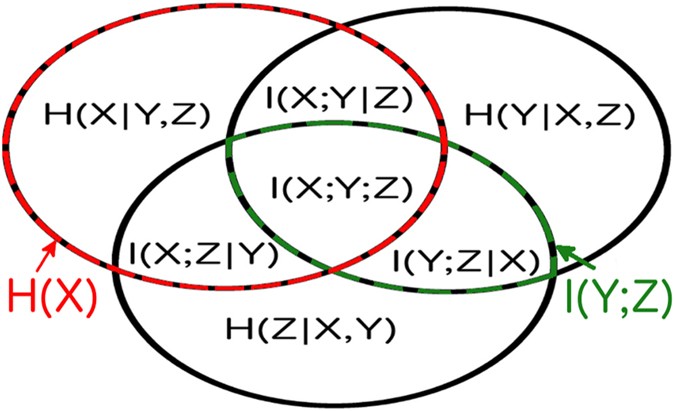
Final Remarks
After reading this post, I hope you have some sense of the information concepts that we have been discussing. Below is one of the Venn diagrams you can find on the internet about this topic. I hope you can understand all the above without looking at this diagram (thus I put it at the last). This and similar diagrams may, however, help when we need some quick reference in the future.