Naive Bayes classifier: a comprehensive guide

Test your knowledge

Naive Bayes is a very popular algorithm in Machine Learning given its simplicity, rigid performance and interesting idea from Bayesian Probability.

In this blog post, we show and explain the Bayes formula, how to build a Naive Bayes classifier (with your pen and paper or with Python-sklearn), the assumptions behind this method together with its strengths and weaknesses.

The curriculum is as below:

Table of content

Naive Bayes method
Example
Laplace smoothing
Naive Bayes with Python
Assumptions
Strengths
Weakness

Naive Bayes method

Naive Bayes classifier algorithm relies on Bayes’ theorem about the probability of an event given prior knowledge related to it. The theorem is simply:

$P(A|B) = \frac{P(B|A)P(A)}{P(B)}$

where:

A and B are 2 events.
$P(A|B)$ is the conditional probability of A given B is true.
$P(B|A)$ is the conditional probability of B given A is true.
$P(A)$ and $P(B)$ are the probabilities of A and B, respectively.

This formula is true because
$P(A|B)P(B) = P(B|A)P(A) = P(A, B)$
(where $P(A, B)$ denotes the joint probability of both events A and B – the probability that both A and B are true).

In the context of Machine Learning and Classification, we can rewrite the formula as below:

$P(c_i|X) = \frac{P(X|c_i)P(c_i)}{P(X)}$

where:

$c_i$ is the i-th class. $1 \leq i \leq k$ with k is the number of classes.
X is the training data. Note that X represents 1 sample data point (not the entire dataset).
$P(c_i|X)$ is the probability that the sample data point X belongs to class i.
$P(X|c_i)$ is the probability of the data point X to appear in class i.
$P(X)$ is the probability of X.

To find the most suitable class for each data point X, we find all the $P(c_i|X)$ for $1 \leq i \leq k$ , and then we assign X to the class with the highest probability.

In other words, we find arg max $_i$ of $P(c_i|X)$ .

Or say, arg max $_i$ of $\frac{P(X|c_i)P(c_i)}{P(X)}$

Notice that the value of $P(X)$ is constant across all classes. So, we can safely ignore it and adjust our goal to finding arg max $_i$ of $P(X|c_i)P(c_i)$ .

$\blacktriangleright$ $P(c_i)$ is easily computed by taking the proportion of class i in our whole dataset.

$P(c_i) = \frac{|X \in c_i|}{n}$ , where n is the sample size and $|X \in c_i|$ is the number of data samples that belong to class i.

$\blacktriangleright$ $P(X|c_i)$ requires a bit more work. Be reminded that X is a vector of values, $X_j$ ( $1 \leq j \leq m$ , where m is the number of predictor variables) is the value of the predictor variable j for this data point X.

We make an assumption here that the predictor variables are all independent of each other.
Thus, $P(X|c_i) = P(X_1|c_i)*P(X_2|c_i)* ... *P(X_m|c_i)$ .

If the j-th predictor variable is a categorical variable, $P(X_j|c_i)$ can be simply calculated from the training dataset. In case it is a numerical variable, we may either distribute the values into bins and then each bin is treated as a categorical value, or assume its distribution (e.g. Gaussian distribution) and then take the PDF.

Example

Suppose our task is to classify the type of animal given its fur color and the sharpness of its claws. The training data looks like below:

Naive Bayes example training data

No.	Fur color	Sharpness of claws	Animal
1	Black	High	Cat
2	Yellow	Low	Cat
3	Black	High	Cat
4	Blue	High	Cat
5	Yellow	Low	Dog
6	Blue	Low	Dog
7	Yellow	High	Dog
8	Black	Low	Dog

and here is the testing data:

Naive Bayes example testing data

No.	Fur color	Sharpness of claws	Animal
9	Yellow	Low	?
10	Black	High	?

We now pre-compute some values with the information provided by the training data. These values are then used to predict the samples in the testing set.

First, we need the probability of each class.

P(Cat) = $\frac{\text{number of cats}}{\text{total sample size}} = \frac{4}{8}$ = 0.5

P(Dog) = $\frac{\text{number of dogs}}{\text{total sample size}} = \frac{4}{8}$ = 0.5

Then, we compute the conditional probability of each category given a class.

P(Fur = Black | Cat) = $\frac{\text{number of cats with black fur}}{\text{number of cats}} = \frac{2}{4} = 0.5$

P(Fur = Black | Dog) = $\frac{\text{number of dogs with black fur}}{\text{number of dogs}} = \frac{1}{4} = 0.25$

P(Fur = Yellow | Cat) = $\frac{\text{number of cats with yellow fur}}{\text{number of cats}} = \frac{1}{4} = 0.25$

P(Fur = Yellow | Dog) = $\frac{\text{number of dogs with yellow fur}}{\text{number of dogs}} = \frac{2}{4} = 0.5$

etc.

Until we have all the conditional probabilities P(category | class) as in the below table.

Naive Bayes example P(category | class)

Class	Fur			Sharpness
	Black	Yellow	Blue	High	Low
Cat	0.5	0.25	0.25	0.75	0.25
Dog	0.25	0.5	0.25	0.25	0.75

We have done the training part. Now, it’s time for predictions. We will predict the classes of 2 testing examples shown above.

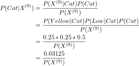
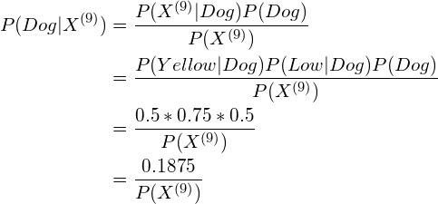
For the first testing sample (the sample with index No. 9):

$\begin{aligned}P(Cat | X^{(9)}) &= \frac{P(X^{(9)}|Cat)P(Cat)}{P(X^{(9)})} \\ &= \frac{ P(Yellow|Cat) P(Low|Cat) P(Cat) }{P(X^{(9)})} \\ &= \frac{0.25 * 0.25 * 0.5}{P(X^{(9)})} \\ &= \frac{0.03125}{P(X^{(9)})} \\\end{aligned}$

$\begin{aligned}P(Dog | X^{(9)}) &= \frac{P(X^{(9)}|Dog)P(Dog)}{P(X^{(9)})} \\ &= \frac{ P(Yellow|Dog) P(Low|Dog) P(Dog) }{P(X^{(9)})} \\ &= \frac{0.5 * 0.75 * 0.5}{P(X^{(9)})} \\ &= \frac{0.1875}{P(X^{(9)})} \\\end{aligned}$

As we know $P(X^{(9)})$ is a positive number (because $P(X^{(9)})$ is the probability of $X^{(9)}$ , and the probability of an already-happened-event is always larger than 0), we have $P(Dog | X^{(9)}) > P(Cat | X^{(9)})$ .

Thus, according to the Naive Bayes algorithm, sample No. 9 is classified as Dog.

For the second testing sample (the sample with index No. 10):

$\begin{aligned}P(Cat | X^{(10)}) &= \frac{P(X^{(10)}|Cat)P(Cat)}{P(X^{(10)})} \\ &= \frac{ P(Black|Cat) P(High|Cat) P(Cat) }{P(X^{(10)})} \\ &= \frac{0.5 * 0.75 * 0.5}{P(X^{(10)})} \\ &= \frac{0.1875}{P(X^{(10)})} \\\end{aligned}$

$\begin{aligned}P(Dog | X^{(10)}) &= \frac{P(X^{(10)}|Dog)P(Dog)}{P(X^{(10)})} \\ &= \frac{ P(Black|Dog) P(High|Dog) P(Dog) }{P(X^{(10)})} \\ &= \frac{0.25 * 0.25 * 0.5}{P(X^{(10)})} \\ &= \frac{0.03125}{P(X^{(10)})} \\\end{aligned}$

Hence, we conclude the sample No.10 is classified as Cat.

Laplace Smoothing

In practice, for categorical variables, it sometimes happens that a category in the testing set does not appear in the training set (e.g. in the above example, what if, in sample No.9, the fur color is Pink instead of Yellow?). In these cases, the results we output are all 0, which gives no clue about which class we should assign the data point to.

To resolve this issue, we often apply Laplace smoothing to the computation of the probabilities.

In other words, instead of the conventional formula:

$P(X_{i} = v_j | c_k) = \frac{n_{ijk}}{n_k}$

we use the Laplace estimate:

$P(X_{i} = v_j | c_k) = \frac{n_{ijk} + 1}{n_k + s_i}$

where:

$X_{i}$ is the value of the sample at the i-th feature.
$v_j$ is the j-th categorical value of feature i.
$c_k$ is the k-th class.
$n_{ijk}$ is the number of samples in $c_k$ that has $X_{i} = v_j$ .
$n_k$ is the number of samples of class k.
$s_i$ is the number of possible values for $X_{i}$ .

For example, if we apply to the problem above:

P(Fur = Black | Cat) = $\frac{\text{cats with black fur + 1}}{\text{cats + 3}} = \frac{2 + 1}{4 + 3} = \frac{3}{7}$

Naive Bayes with Python

To run the Naive Bayes algorithm in Python, we could use the pre-built functions from sklearn library, which can be found in sklearn.naive_bayes:

sklearn.naive_bayes.CategoricalNB: for using Naive Bayes on categorical predictor variables, just like we did in the example above.
sklearn.naive_bayes.GaussianNB: for Naive Bayes on numerical predictor variables, with the assumption that these variables follow Gaussian distribution.
sklearn.naive_bayes.MultinomialNB: the predictor variables represent the counts, a popular application is in text classification. Fractional counts like tf-idf may also work.
sklearn.naive_bayes.ComplementNB: A modification of MultinomialNB which is suitable for imbalanced datasets.
sklearn.naive_bayes.BernoulliNB: assumes the data follows Bernoulli distribution (i.e. possible values of predictor variables are 0 and 1).

Assumptions

Features (predictor variables) are independent of each other.
The solution for handling continuous data (binning or assuming a distribution) is suitable.

Strengths

Surprisingly simple. It is just counting the values.
Naive Bayes is a generative model. It is comfortable with just a small amount of data.
It is fast and requires less Memory.
Moderate performance in general, even better if the assumptions hold.
Innate ability to handling missing value (just ignore that feature).
Output probabilistic predictions (i.e. it does not just classify the data but even produces numerical values representing how likely a data point belongs to each class).
Naive Bayes is not sensitive to noisy data.

Weaknesses

The assumption of feature independent rarely holds true.
It is quite hard to handle continuous feature properly.
Naive Bayes treats each feature independently, thus it does not learn the interaction between features. For example, Tony does not want to go outside when he is in a bad mood or it is raining, but he likes to go out if both conditions are true.
The performance is not the best (compared to other algorithms) in most cases.
Do not support online-learning. When you have new data, you have to re-train the Naive Bayes model.
Do not work (well) if some values in the testing set do not appear in the training set.

Test your understanding

References:

Toronto Naive Bayes Classification Lecture 3: link
Wiki – Naive Bayes classifier: link
Scikit-learn Naive Bayes: link
Quora – Advantages of Naive Bayes: link
Edwin Chen’s Blog about Classifiers: link

Tung M Phung's Blog

Naive Bayes classifier: a comprehensive guide

Naive Bayes example training data

Naive Bayes example testing data

Naive Bayes example P(category | class)

Leave a ReplyCancel reply