
A window function performs the calculation of each row over a set of rows (a group / a partition / a window of rows) that they belong to.
For example, assume we have a table containing information about students in your school. The information stored includes major, class ID, gender, date of birth, score, etc. Now, we want to have the relative ranking of every student’s score in his/her class, what should we do?
This is a perfect chance for a window function to take action! What the window function does is: partition the students into class, then for each class, apply the RANK() function. Simple, isn’t it?
Apart from RANK(), there are also other window functions that are very useful. Let’s take a look at them together (, but later, after the following example).
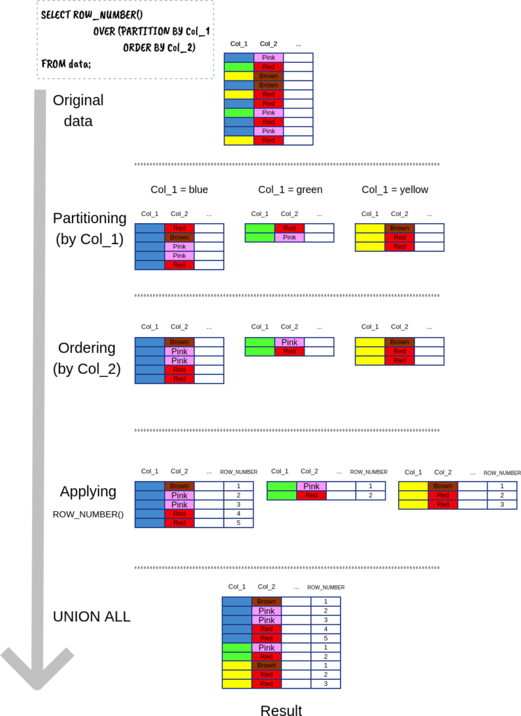
The ROW_NUMBER() window function helps to assign a unique index for each row in a partition, follow a specified ordering scheme. The process is fully explained by the below visual.
List of window functions
ROW_NUMBER(): row-count within its partition (from 1 to n). Example.
RANK(): the rank of the current row in its partition, with gaps. E.g. RANK() on [-3, 2, 2, 6, 8, 8] gives [1, 2, 2, 4, 5, 5]. Example.
DENSE_RANK(): the rank of the current row in its partition, without gaps. E.g. RANK() on [-3, 2, 2, 6, 8, 8] gives [1, 2, 2, 3, 4, 4]. Example.
PERCENT_RANK(): equals to applying a RANK() and then normalize the values to the range [0, 1] (i.e. equal (rank – 1) / (number of rows in partition – 1)). Example.
CUME_DIST(): the cumulative distribution. It equals (the number of rows smaller than or equal to it, including itself) / (the total number of rows in its partition). Example.
NTILE(n_buckets): each partition is divided into a number of buckets, then all rows belonging to a bucket is marked by the index number of that bucket. If the number of rows is not divisible by the number of buckets, bucket sizes will have a difference of at most 1, while the bigger buckets precede the smaller ones. Example.
LAG(expression, offset, default value): return the expression evaluated at the row that is offset rows before the current row. If that row does not exist, the default value will be returned. If not specified, offset is 1 and the default value is NULL. Example.
LEAD(expression, offset, default value): return the expression evaluated at the row that is offset rows after the current row. If that row does not exist, the default value will be returned. If not specified, offset is 1 and the default value is NULL. Example.
FIRST_VALUE(expression): the expression evaluated at the first row of the partition (the window). Caution. Example.
LAST_VALUE(expression): the expression evaluated at the last row of the partition (the window). Caution. Example.
NTH_VALUE(express, n-th): the expression evaluated at the n-th row of the partition (the window). NULL is returned if no such row. Caution. Example.
Caution: FIRST_VALUE, LAST_VALUE, and NTH_VALUE, by default, only consider the window from the start of the partition to the last peer of the current row. This works well for FIRST_VALUE, however, it may induce some NULL for NTH_VALUE and some wrong values for LAST_VALUE. To solve the problem, add RANGE BETWEEN UNBOUNDED PRECEDING AND UNBOUNDED FOLLOWING into the OVER clause. See example and example.
Notes:
Aggregate functions as window functions
All the aggregate functions (SUM, COUNT, MIN, MAX, etc.) can be used as window functions as well. The keyword is OVER.
For example, we may use the ARRAY_AGG either by the syntax:
SELECT ARRAY_AGG(expression_1) OVER (PARTITION BY expression_2);
or:
SELECT ARRAY_AGG(expression_1) OVER (PARTITION BY expression_2 ORDER BY expression_3);
What is the difference? That is about the window. For the first syntax, the window for executing each row is the entire partition. For the second syntax, the window for executing each row includes rows from the start of the partition to the last peer of the current row.
Take a look at the 2 syntaxes in action:
SELECT inventory_id AS inventory
     , customer_id AS customer
     , EXTRACT(MONTH FROM rental_date) AS month
     , ARRAY_AGG(customer_id) OVER (PARTITION BY inventory_id) AS ARR
FROM rental
LIMIT 10;
| inventory | customer | month | arr |
|---|---|---|---|
| 1 | 279 | 8 | {279,518,431} |
| 1 | 518 | 8 | {279,518,431} |
| 1 | 431 | 7 | {279,518,431} |
| 2 | 359 | 8 | {359,581,161,170,411} |
| 2 | 581 | 7 | {359,581,161,170,411} |
| 2 | 161 | 7 | {359,581,161,170,411} |
| 2 | 170 | 6 | {359,581,161,170,411} |
| 2 | 411 | 5 | {359,581,161,170,411} |
| 3 | 541 | 8 | {541,39} |
| 3 | 39 | 7 | {541,39} |
SELECT inventory_id AS inventory
     , customer_id AS customer
     , EXTRACT(MONTH FROM rental_date) AS month
     , ARRAY_AGG(customer_id) OVER (PARTITION BY inventory_id
                                    ORDER BY EXTRACT(MONTH FROM rental_date))
                              AS ARR
FROM rental
LIMIT 10;
| inventory | customer | month | arr |
|---|---|---|---|
| 1 | 431 | 7 | {431} |
| 1 | 518 | 8 | {431,518,279} |
| 1 | 279 | 8 | {431,518,279} |
| 2 | 411 | 5 | {411} |
| 2 | 170 | 6 | {411,170} |
| 2 | 581 | 7 | {411,170,581,161} |
| 2 | 161 | 7 | {411,170,581,161} |
| 2 | 359 | 8 | {411,170,581,161,359} |
| 3 | 39 | 7 | {39} |
| 3 | 541 | 8 | {39,541} |
Examples:
For illustrative purposes, we will be using the Pagila database, which is a port of the Sakila database (for MySQL) to Postgresql – the SQL version of this blog post. Pagila can be downloaded from here.
Example ROW_NUMBER:
SELECT inventory_id
     , rental_date
     , ROW_NUMBER() OVER (PARTITION BY inventory_id ORDER BY rental_date)
FROM rental
LIMIT 10;
| inventory_id | rental_date | row_number |
|---|---|---|
| 1 | 2005-07-08 19:03:15 | 1 |
| 1 | 2005-08-02 20:13:10 | 2 |
| 1 | 2005-08-21 21:27:43 | 3 |
| 2 | 2005-05-30 20:21:07 | 1 |
| 2 | 2005-06-17 20:24:00 | 2 |
| 2 | 2005-07-07 10:41:31 | 3 |
| 2 | 2005-07-30 22:02:34 | 4 |
| 2 | 2005-08-23 01:01:01 | 5 |
| 3 | 2005-07-31 21:36:07 | 1 |
| 3 | 2005-08-22 23:56:37 | 2 |
Example RANK:
SELECT staff_id
     , payment_date
     , RANK() OVER (PARTITION BY staff_id ORDER BY payment_date)
FROM payment
LIMIT 10;
| staff_id | payment_date | rank |
|---|---|---|
| 1 | 2017-01-24 21:21:56 | 1 |
| 1 | 2017-01-24 21:21:56 | 1 |
| 1 | 2017-01-24 21:33:07 | 3 |
| 1 | 2017-01-24 21:33:07 | 3 |
| 1 | 2017-01-24 21:33:47 | 5 |
| 1 | 2017-01-24 21:33:47 | 5 |
| 1 | 2017-01-24 21:36:33 | 7 |
| 1 | 2017-01-24 21:36:33 | 7 |
| 1 | 2017-01-24 22:29:06 | 9 |
| 1 | 2017-01-24 22:29:06 | 9 |
Example DENSE_RANK:
SELECT staff_id
     , payment_date
     , DENSE_RANK() OVER (PARTITION BY staff_id ORDER BY payment_date)
FROM payment
LIMIT 10;
| staff_id | payment_date | dense_rank |
|---|---|---|
| 1 | 2017-01-24 21:21:56 | 1 |
| 1 | 2017-01-24 21:21:56 | 1 |
| 1 | 2017-01-24 21:33:07 | 2 |
| 1 | 2017-01-24 21:33:07 | 2 |
| 1 | 2017-01-24 21:33:47 | 3 |
| 1 | 2017-01-24 21:33:47 | 3 |
| 1 | 2017-01-24 21:36:33 | 4 |
| 1 | 2017-01-24 21:36:33 | 4 |
| 1 | 2017-01-24 22:29:06 | 5 |
| 1 | 2017-01-24 22:29:06 | 5 |
Example PERCENT_RANK:
SELECT staff_id
     , payment_date
     , PERCENT_RANK() OVER (PARTITION BY staff_id ORDER BY payment_date)
FROM payment
LIMIT 10;
| staff_id | payment_date | percent_rank |
|---|---|---|
| 1 | 2017-01-24 21:21:56 | 0 |
| 1 | 2017-01-24 21:21:56 | 0 |
| 1 | 2017-01-24 21:33:07 | 1.2491412154144027E-4 |
| 1 | 2017-01-24 21:33:07 | 1.2491412154144027E-4 |
| 1 | 2017-01-24 21:33:47 | 2.4982824308288055E-4 |
| 1 | 2017-01-24 21:33:47 | 2.4982824308288055E-4 |
| 1 | 2017-01-24 21:36:33 | 3.7474236462432077E-4 |
| 1 | 2017-01-24 21:36:33 | 3.7474236462432077E-4 |
| 1 | 2017-01-24 22:29:06 | 4.996564861657611E-4 |
| 1 | 2017-01-24 22:29:06 | 4.996564861657611E-4 |
Example CUME_DIST:
SELECT staff_id
     , payment_date
     , CUME_DIST() OVER (PARTITION BY staff_id ORDER BY payment_date)
FROM payment
LIMIT 10;
| staff_id | payment_date | cume_dist |
|---|---|---|
| 1 | 2017-01-24 21:21:56 | 1.2490632025980515E-4 |
| 1 | 2017-01-24 21:21:56 | 1.2490632025980515E-4 |
| 1 | 2017-01-24 21:33:07 | 2.498126405196103E-4 |
| 1 | 2017-01-24 21:33:07 | 2.498126405196103E-4 |
| 1 | 2017-01-24 21:33:47 | 3.7471896077941546E-4 |
| 1 | 2017-01-24 21:33:47 | 3.7471896077941546E-4 |
| 1 | 2017-01-24 21:36:33 | 4.996252810392206E-4 |
| 1 | 2017-01-24 21:36:33 | 4.996252810392206E-4 |
| 1 | 2017-01-24 22:29:06 | 6.245316012990258E-4 |
| 1 | 2017-01-24 22:29:06 | 6.245316012990258E-4 |
Example NTILE:
SELECT inventory_id
     , rental_date
     , NTILE(2) OVER (PARTITION BY inventory_id ORDER BY rental_date)
FROM rental
LIMIT 10;
| inventory_id | rental_date | ntile |
|---|---|---|
| 1 | 2005-07-08 19:03:15 | 1 |
| 1 | 2005-08-02 20:13:10 | 1 |
| 1 | 2005-08-21 21:27:43 | 2 |
| 2 | 2005-05-30 20:21:07 | 1 |
| 2 | 2005-06-17 20:24:00 | 1 |
| 2 | 2005-07-07 10:41:31 | 1 |
| 2 | 2005-07-30 22:02:34 | 2 |
| 2 | 2005-08-23 01:01:01 | 2 |
| 3 | 2005-07-31 21:36:07 | 1 |
| 3 | 2005-08-22 23:56:37 | 2 |
Example LAG:
SELECT inventory_id
     , rental_date
     , LAG(rental_date, 1) OVER (PARTITION BY inventory_id ORDER BY rental_date) AS previous_rent
FROM rental
LIMIT 10;
| inventory_id | rental_date | previous_rent |
|---|---|---|
| 1 | 2005-07-08 19:03:15 | |
| 1 | 2005-08-02 20:13:10 | 2005-07-08 19:03:15 |
| 1 | 2005-08-21 21:27:43 | 2005-08-02 20:13:10 |
| 2 | 2005-05-30 20:21:07 | |
| 2 | 2005-06-17 20:24:00 | 2005-05-30 20:21:07 |
| 2 | 2005-07-07 10:41:31 | 2005-06-17 20:24:00 |
| 2 | 2005-07-30 22:02:34 | 2005-07-07 10:41:31 |
| 2 | 2005-08-23 01:01:01 | 2005-07-30 22:02:34 |
| 3 | 2005-07-31 21:36:07 | |
| 3 | 2005-08-22 23:56:37 | 2005-07-31 21:36:07 |
Example LEAD:
SELECT inventory_id
     , rental_date
     , LEAD(rental_date, 1) OVER (PARTITION BY inventory_id ORDER BY rental_date) AS next_rent
FROM rental
LIMIT 10;
| inventory_id | rental_date | next_rent |
|---|---|---|
| 1 | 2005-07-08 19:03:15 | 2005-08-02 20:13:10 |
| 1 | 2005-08-02 20:13:10 | 2005-08-21 21:27:43 |
| 1 | 2005-08-21 21:27:43 | |
| 2 | 2005-05-30 20:21:07 | 2005-06-17 20:24:00 |
| 2 | 2005-06-17 20:24:00 | 2005-07-07 10:41:31 |
| 2 | 2005-07-07 10:41:31 | 2005-07-30 22:02:34 |
| 2 | 2005-07-30 22:02:34 | 2005-08-23 01:01:01 |
| 2 | 2005-08-23 01:01:01 | |
| 3 | 2005-07-31 21:36:07 | 2005-08-22 23:56:37 |
| 3 | 2005-08-22 23:56:37 |
Example FIRST_VALUE:
SELECT inventory_id
     , rental_date
     , FIRST_VALUE(rental_date) OVER (PARTITION BY inventory_id ORDER BY rental_date) AS first_rent
FROM rental
LIMIT 10;
| inventory_id | rental_date | first_rent |
|---|---|---|
| 1 | 2005-07-08 19:03:15 | 2005-07-08 19:03:15 |
| 1 | 2005-08-02 20:13:10 | 2005-07-08 19:03:15 |
| 1 | 2005-08-21 21:27:43 | 2005-07-08 19:03:15 |
| 2 | 2005-05-30 20:21:07 | 2005-05-30 20:21:07 |
| 2 | 2005-06-17 20:24:00 | 2005-05-30 20:21:07 |
| 2 | 2005-07-07 10:41:31 | 2005-05-30 20:21:07 |
| 2 | 2005-07-30 22:02:34 | 2005-05-30 20:21:07 |
| 2 | 2005-08-23 01:01:01 | 2005-05-30 20:21:07 |
| 3 | 2005-07-31 21:36:07 | 2005-07-31 21:36:07 |
| 3 | 2005-08-22 23:56:37 | 2005-07-31 21:36:07 |
Example LAST_VALUE:
SELECT inventory_id
     , rental_date
     , LAST_VALUE(rental_date) OVER (PARTITION BY inventory_id ORDER BY rental_date
                                     RANGE BETWEEN UNBOUNDED PRECEDING
                                               AND UNBOUNDED FOLLOWING)
                               AS last_rent
FROM rental
LIMIT 10;
| inventory_id | rental_date | last_rent |
|---|---|---|
| 1 | 2005-07-08 19:03:15 | 2005-08-21 21:27:43 |
| 1 | 2005-08-02 20:13:10 | 2005-08-21 21:27:43 |
| 1 | 2005-08-21 21:27:43 | 2005-08-21 21:27:43 |
| 2 | 2005-05-30 20:21:07 | 2005-08-23 01:01:01 |
| 2 | 2005-06-17 20:24:00 | 2005-08-23 01:01:01 |
| 2 | 2005-07-07 10:41:31 | 2005-08-23 01:01:01 |
| 2 | 2005-07-30 22:02:34 | 2005-08-23 01:01:01 |
| 2 | 2005-08-23 01:01:01 | 2005-08-23 01:01:01 |
| 3 | 2005-07-31 21:36:07 | 2005-08-22 23:56:37 |
| 3 | 2005-08-22 23:56:37 | 2005-08-22 23:56:37 |
Example NTH_VALUE:
SELECT inventory_id
     , rental_date
     , NTH_VALUE(rental_date, 2) OVER (PARTITION BY inventory_id ORDER BY rental_date
                                       RANGE BETWEEN UNBOUNDED PRECEDING
                                                 AND UNBOUNDED FOLLOWING)
                                 AS second_rent
FROM rental
LIMIT 10;
| inventory_id | rental_date | second_rent |
|---|---|---|
| 1 | 2005-07-08 19:03:15 | 2005-08-02 20:13:10 |
| 1 | 2005-08-02 20:13:10 | 2005-08-02 20:13:10 |
| 1 | 2005-08-21 21:27:43 | 2005-08-02 20:13:10 |
| 2 | 2005-05-30 20:21:07 | 2005-06-17 20:24:00 |
| 2 | 2005-06-17 20:24:00 | 2005-06-17 20:24:00 |
| 2 | 2005-07-07 10:41:31 | 2005-06-17 20:24:00 |
| 2 | 2005-07-30 22:02:34 | 2005-06-17 20:24:00 |
| 2 | 2005-08-23 01:01:01 | 2005-06-17 20:24:00 |
| 3 | 2005-07-31 21:36:07 | 2005-08-22 23:56:37 |
| 3 | 2005-08-22 23:56:37 | 2005-08-22 23:56:37 |
References: