
Last time, we introduced Z-score and the Z-family. Today, we visit another house to meet the family of the T, consisting of T-statistic, T-test, T-distribution, etc.
Definition of the T-
The T-family is very similar to the Z-family, it acts as a substitution or approximation for the Z-family in some cases.
Depending on the input that we choose to use the Z- or the T-. We use T-family when:
- We don’t know the true variance of the distribution that the sample(s) is drawn from, or
- the sample size is
 30.
30.
otherwise, we use Z-family.
T-test
T-test refers to any hypothesis test that its result follows a T-distribution.
In practice, the tests are usually about the mean of 1 or 2 sample sets.
There are crucially 3 types of T-tests, those are:
One-sample T-test
‘One-sample‘ here does not mean a sample set of size 1, be careful, it is a bit confusing! In fact, this test is about one set of samples (with set size  2).
2).
Formally, One-sample T-test tests whether the mean of a sample set ( ) is significantly different from a population mean (
 ) or not.
The hypothesis test’s structure is:

If you are familiar with Z-test, you will catch up with the T-test right away, because they are really close.
First, we compute the t-statistic (t):

with degree of freedom (d.f) = n-1.
The formula of t-statistic is comparable to that of z-statistic, with 2 differences:
- Use sample standard deviation (s) instead of population standard deviation (
 ). This is because we do not know the value of , thus s is used as an approximation.
 - There is a new term: the degree of freedom (explanation in Appendix A).
Example:
We have a set of 4 sample data points and their values are 20, 40, 55, 30. Hence, our sample mean is 36.25 and the standard deviation of  12.93. We want to test the hypothesis that this sample set is sampled from a population with the mean 40, the significance level (
 ) for this test is 0.1.
We don’t know the population’s standard deviation, and even more, the sample size is not greater than 30, thus we use the T-test instead of the Z-test. In fact, both conditions for using the T-test are satisfied, while we need just 1 to decide to use the T-test in favor of the Z-test.
We compute the t-statistic and degree of freedom:
t 
d.f = 4 – 1 = 3
When we obtained the t-statistic and the degree of freedom, it’s time to look up the critical value using t-table (Appendix B) or using Python (Appendix C). The critical value is a number represents how extreme our t-statistic should be so that we can reject the Null hypothesis. In other words, if our t-statistic is the critical value, we reject the Null hypothesis.
With input: = 0.1, 2-tailed test, d.f = 3; we get the critical value = 2.353. Because our t-statistic is 0.58, smaller than this critical value, we end up accepting the Null Hypothesis that the sample mean is quite similar (or says, not statistically different) to 40.
| Test your understanding |
|
|
Conclusion
This blog post gives an overview of the T-family. Essentially, T-family is used in place of the Z-family when the number of sample data points is small or when we don’t know the population variance.
One-sample T-test is a T-test that examines one set of sample data, as opposed to Paired-sample and Unpaired-sample T-tests, while there are 2 sets of samples in execution. One-sample T-test is introduced in this blog post, on the other hand, the remaining 2 are in the subsequent post on the T-family.
References:
- Wikipedia’s page about Student t-test: link
- The T-table from Stanford University: link
- Scipy.stats: link
Appendix A: Degree of freedom
Degree of freedom is the number of parameters that can vary but the proposed properties can still hold. For example, we have a set of 5 numbers (from  to
to  ) with known mean equals 10. We can change the value of 4 numbers in these 5 to any values we want, then the property of mean equals 10 can still hold if we set the fifth-number to be equal
  (sum of the other 4 numbers). If we vary the value of all 5 numbers, the property of mean equals 10 might not hold. Thus, the degree of freedom in this example is 4.
Formula to get the degree of freedom of a set of n samples (and we DO know the mean of this set) is:
d.f = n – 1
Appendix B: Testing hypotheses with T-table
Reading the T-table may be a little bit different from the Z-table.
For the Z-table, we use our z-score to find the corresponding percentile (p-value) on the table. If this percentile is smaller than the significance level (), we reject the Null Hypothesis. However, with the T-table, we use the degree of freedom and the significance level to get the critical value. If our t-statistic is larger than this critical value, then we reject the Null Hypothesis. If our t-statistic is smaller than this critical value, we failed to reject the Null Hypothesis.
This is a T-table:
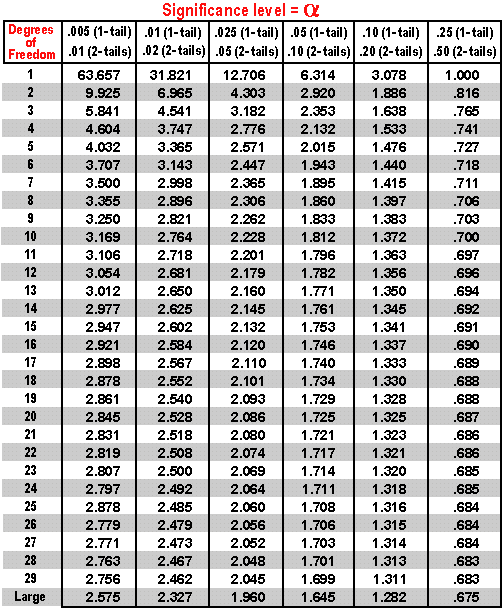
For example, we want to make a one-sided T-test with the significance level = 0.05 and have the computed t-statistic = 2.6 and degree of freedom = 20. Lookup the T-table on this d.f and , we see the critical value of 1.725, which is smaller than our real t-statistic 2.6. Hence, we conclude that we reject the Null Hypothesis and accept the Alternative Hypothesis.
Appendix C: Testing hypotheses with Python
Python’s Scipy library supports a function to query the critical value, which works just like we look up in the T-table. We should input 2 values: one minus and the degree of freedom, then the function will output the critical value.
For example, if our = 0.05, an 1-tailed test, with d.f = 20, then we call:
from scipy import stats
print(stats.t.ppf(1-0.05, 20))
| 1.7247182429207857 |
With the same example, if we use a 2-tailed test, the call would be:
from scipy import stats
print(stats.t.ppf(1-0.05/2, 20))
| 2.0859634472658364 |