Unpaired Two-sample T-test (Independent T-test)

Test your knowledge

What is an Unpaired 2-sample T-test?

Let’s analyze this definition from scratch. A T-test is a statistical test whose outcomes follow a T-distribution. Two-sample means we have 2 sets of samples, and our target is to verify if the means of the 2 distributions that generate these 2 sample sets are equal. Unpaired means these 2 sample sets are independent of each other, each observation in one sample set does NOT correspond to one and only one observation in the other set (it is opposite to the case of Paired Test). Thus, in summary, an Unpaired 2-sample T-test takes as input 2 sample sets that are independent of each other, and the test’s outputs follow a T-distribution. This is also abbreviated as an Unpaired T-test or Independent T-test.

In contrast to the Unpaired 2-sample T-test, we also have the Paired 2-sample T-test.

	Paired 2-sample T-test	Unpaired 2-sample T-test
Usage	When each observation in a sample set is semantically related to one and only one observation in the other set.	When the requirement of correspondence for the Paired 2-sample T-test does not hold.
Usecase examples	We have a soft-skill course. We measure the performance of our company’s employees before and after learning the course to see if this course enhances employee productivity. We do A/B Testing on our ads. For each of our webpages, blue-colored theme ads are shown for some guests while yellow-colored theme ads are shown to the others. After a day, we have 2 sets of sample data, one contains the average click-through rate (for ads) of each webpage when blue ads are shown, the other contains the same measure for yellow ads. We compare these 2 sets to see if one color is significantly more attractive than the other.	There are 2 sample sets, one is the weights of 30 men and the other is the weights of 30 women. We want to test if the weight is significantly different for different genders. We do A/B Testing on our ads. For some random webpages, we show ads with blue-colored themes, while for the other webpages, yellow-colored theme ads are shown. After a day, we have 2 sets of sample data, one contains the average click-through rate (for ads) of each webpage that is attached with blue ads, the other contains the same measure for webpages with yellow ads. We compare these 2 sets to see if one color is significantly more attractive than the other.
Sample sizes	The sizes of the 2 sample sets must be the same.	2 sample sets may have different sizes.

Notice that the result taken from the Paired Test is more significant than from the Unpaired Test given the same samples (because the 1-to-1 relationship gives additional information), it is recommended to take the Paired Test if possible (i.e. if the conditions for a Paired Test hold).

Assumptions

All T-tests are parametric tests, so they do require some assumptions to be at least approximately true.

The observations must be measured in numerical values (i.e. continuous, interval or ratio). For categorical variables, we should use another test, for example, the Chi-squared test.
Both distributions that generate the 2 sample sets must be Normal distributions. This normality can be roughly verified by examining the observations using, for instance, QQ-plot, Shapiro-Wilk or Anderson Darling test. For non-normal data, we can either try to transform it to normal or use a non-parametric test, e.g. Mann Whitney Test and Wilcoxon Signed Rank Test.
Each observation must be independent of any others in both sample sets. Dependencies between observations may affect the objectivity of the test, which makes the test result unreliable. The assumption of independence between observations is almost always attached to all, including both parametric and non-parametric tests.
There must not be any big-influencers (outliers). Outliers may bias the test, especially when the sample size is small (, which case is often for medical tests). In cases there are big-influencers in our data, we may choose to remove it (with care) or switch to a robust test like the Wilcoxon Signed Rank Test, which calculates the ranking thus is not impacted so much by extreme values.
The variances of the 2 distributions that generate the 2 sample sets must be assumed equal. If the variances are not equal, but all the other assumptions still hold, then we could refer to the Welch’s t-test.

Note that even though the tests’ general goal is to check if the means of the 2 distributions are equal or not, it is usually the case that it checks whether the 2 distributions are the same or not. That is, we usually assume the variances of the 2 distribution are equal, then we test if the means are also equal (both the means and variances are equal indicates that the 2 distributions are also the same) or not (implies that 2 distributions are not the same).

Conduct the Test

As the formula for an Unpaired T-test may be a bit involved, to understand it clearly, that would be better if we could rehearse our knowledge.

As we learned before, the T-test is created to be a substitution of the Z-test in cases we do not know the population variance. To compensate for this lack of knowledge, we define a parameter called the degree of freedom (DF), which is linearly correlated with the sample size. If a Normal distribution is formed by just $\mu$ and $\sigma^2$ , a T-distribution is formed by $\mu$ , $\sigma^2$ and DF. The bigger the sample size, the higher the DF, thus the more similar the T-distribution at that DF to the Normal distribution. (In practice, when DF > 30, we consider the Normal and the T-distribution are the same.) The reason for this is because a high DF means a high sample size, which in turn indicates that the sample set better represents the whole population.

Demonstration of how different DFs affect the shape of T-distribution. The higher the DF, the more similar the T-distribution is to the Normal distribution. The figure is taken from Financetrain.

A low-DF T-distribution has a fatter tail because when the sample size is small, we are more cautious with using it as the representative of the population, i.e. we expect more weird things to come when using a small set.

That said, the T-distribution is used as a more cautious version of the Normal distribution when the data size is small. So every computation we use in any T-test has its root in Z-test and can be related back to a Z-test just by switching from the T-distribution to Normal distribution.

The simplest Z-score formula is:

$\begin{aligned}\text{Z-score(x)} = \frac{x - \mu}{\sigma}\end{aligned}$

which is simply the signed distance from the value x to the mean $\mu$ of the population, with unit $\sigma$ .

All other tests, including One-sample and Two-sample tests, are just extended from this formula. In One-sample T-test, for example, the T-score is computed by:

$\begin{aligned}T = \frac{\overline{x} - \mu}{s / \sqrt{n}}\end{aligned}$

with the numerator kept intuitively the same, while the denominator is also the standard deviation, however, it is the standard deviation of the sample set of size n, since we examine a set of sample data instead of one sample data point alone.

For the Independent Two-sample T-test, the idea is not changing at all. Let us write the formula out first and then explain it right after. Be noted that, for simplicity, we consider the case when the 2 sample sizes are equal and the 2 population variances are also assumed equal.

$\begin{aligned}T = \frac{\overline{X_1} - \overline{X_2}}{s_p \sqrt{\frac{2}{n}}}, DF = 2n - 2\end{aligned}$

where:

$\overline{X_1}$ is the mean of the first set,
$\overline{X_2}$ is the mean of the second set,
$s_p$ is the standard deviation of this pair, or say, the pooled standard deviation. $s_p = \sqrt{\frac{s_1^2 + s_2^2}{2}}$ (to be explained below).
$s_1$ and $s_2$ are the standard deviations of the 2 sets, respectively.
n is the size of each sample set.

The numerator is the difference between 2 means, just like the original from Z-score. However, in this problem, we do not have a population mean, instead, we have only 2 sample sets, so we take the difference between their means.

The denominator is a bit more complex. $s_p$ is the standard deviation of the pair. The Variance of the pair is taken to be the average variance of these 2 sets, and then the standard deviation of the pair, $s_p$ is gotten as the square-root of the Variance, thus we have the above formula for $s_p$ .

$s_p$ is then be divided by $\sqrt{n}$ , which is similar to in One-sample Test, the reason is that we are examining samples of size n instead of 1 observation alone.

Lastly, the denominator is multiplied by $\sqrt{2}$ . This is because we are dealing with 2 sample sets instead of 1, the variance between those 2 sets, in the worst case when they are varying in the opposite directions, maybe double of the variance between 1 sample set and the formal, perfect, whole population.

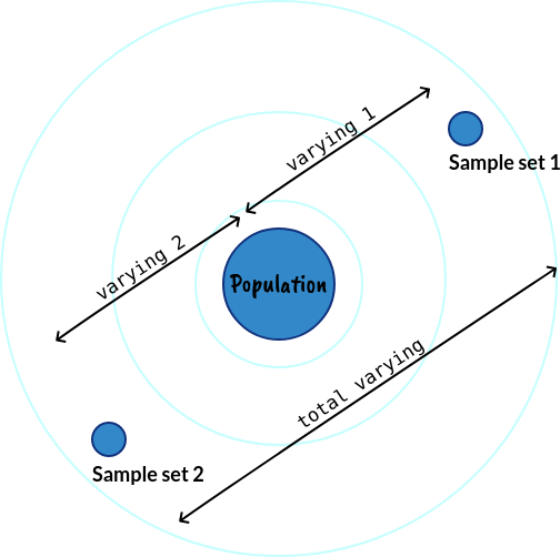
In the worst-case scenario, the 2 sample sets vary from the population in opposite directions. To take care of this, we need to set the Variance of pair equal the sum of their variances.

This also complies with a well-known property of variance: the variance is additive when the 2 datasets are independent of each other.

The degree of freedom equals 2n – 2 as the total number of observations is 2n and we know the 2 means of the sets.

To sum up, we conclude that the formula for T-score in the Independent Two-sample T-test keeps the same form as its root from the Z-test, which is: the difference of means divided by standard deviation, with just some modification to adapt to the input (2 independent sample sets). Overall, the idea is unaltered.

What if the sample sizes are not equal ( $n_1 \neq n_2$ )?

In that case, the computation of the denominator (the standard deviation) should be affected, since each sample set has a different degree of effect to the overall std. (On a side note, literature usually calls the standard deviation of a sample set as the standard error (SE).)

$\begin{aligned}T = \frac{\overline{X_1} - \overline{X_2}}{s_p \sqrt{\frac{1}{n_1} + \frac{1}{n_2}}}, DF = n_1 + n_2 - 2\end{aligned}$

where:

$\begin{aligned}s_p = \sqrt{\frac{(n_1 - 1)s_{X_1}^2 + (n_2 - 1)s_{X_2}^2}{n_1 + n_2 - 2}}\end{aligned}$

$s_p$ is the pooled standard deviation (or overall standard deviation), which is the square root of the pooled variance. Intuitively, the pooled variance is nothing more than a weighted-average of the 2 sample variances with weighting depends on sizes of the samples.

Notice that this pooled standard deviation is just the standard deviation of one observation. What we need here is the standard deviation of a set of samples (this set is a combination of the 2 original sample sets), or say the standard error. Thus, we multiple the pooled standard deviation with $\sqrt{\frac{1}{n_1} + \frac{1}{n_2}}$ .

If $n_1 = n_2$ , this formula boils down exactly to the above when we assume the 2 sample sizes are equal.

After getting the T-statistics and the degree of freedom, we can verify our hypothesis using the T-table (or with the help of Python, or other means) as previously described here.

Example

We want to test whether a new medicine is more effective in reducing blood pressure than the current one. We do an experiment on some patients, with group 1 using the current state-of-the-art treatment while the second group is treated with the novel drug. The hypothesis test structure is formulated as:

$H_0: \overline{X_1} = \overline{X_2}$
$H_1: \overline{X_1} < \overline{X_2}$

and the significance level is set to be 0.05.

After 3 months of consuming the drugs, the amount of reduced blood pressure for the 2 groups is:

$X_1$ = {5, 3, 6, 5, 4, 7, 6, 4, 5, 6, 2, 5}. $n_1$ = 12.
$X_2$ = {8, 11, 7, 9, 10, 8, 6, 9, 10, 8, 7, 9 , 5}. $n_2$ = 13.

With this input at hand, we then compute the required values:

$\begin{aligned}&\overline{X_1} \approx 4.83 \\&\overline{X_2} \approx 8.23 \\&s_{X_1} = \sqrt{\sum_{1 \leq i \leq n_1} \frac{(X_1^{(i)} - \overline{X_1})^2}{n_1 - 1}} \approx 1.403 \\&s_{X_2} = \sqrt{\sum_{1 \leq i \leq n_2} \frac{(X_2^{(i)} - \overline{X_2})^2}{n_2 - 1}} \approx 1.691 \\&s_p = \sqrt{\frac{(n_1 - 1)s_{X_1}^2 - (n_2 - 1)s_{X_2}^2}{n_1 + n_2 - 2}} \approx 1.56 \\&T = \frac{\overline{X_1} - \overline{X_2}}{s_p \sqrt{\frac{1}{n_1} + \frac{1}{n_2}}} \approx -5.44 \\&DF = n_1 + n_2 - 2 = 23\end{aligned}$

Looking up the T-table on $\alpha = 0.05$ for 1-tailed T-test with DF = 23 gives the Critical value = 1.714, thus for our alternative hypothesis to be true, we need the absolute of T-statistic to be higher than 1.714, which is fulfilled. Hence, we conclude that we reject the Null Hypothesis to accept the Alternative Hypothesis.

Test your understanding

References:

Wikipedia’s page about Student T-test: link
Wikipedia’s page about Pooled Variance: link
a post on statisticshowto about Independent T-test: link
a post on Spss-tutorials about Independent T-test: link
a chapter about Two-Sample T-test on Nist: link
Hypothesis Testing with Two Samples Exercise on Libretexts: link
Paired and Independent T-test Exercise on Eagri: link

Tung M Phung's Blog

Unpaired Two-sample T-test (Independent T-test)

Leave a ReplyCancel reply